This simulation compares the Type I (false positive) error rate for analyses with and without covariates. It demonstrates the effect on the Type I error rate when both unadjusted and covariate-adjusted analyses are performed and only the smallest p-value is reported, and it demonstrates how the magnitude of the correlation between variables in the analysis (the outcome variable and up to two covariates) affects these results.
The workhorse of the script is the run.sim function, which takes 4 parameters:
n.sims: Size of simulation, that is, the number of experiments to simulate.N: Number of observations per experiment. Must be an even number.corr: The correlation between variables (outcome and up to 2 covariates) in the experiment. May be 0, in which case variables will be independent.seed: Non-negative integer to seed the pseudo random number generator. Set to 0 to allow the computer to pick the seed, or to a positive integer to produce reproducible results.run.sim performs a simulation comprising n.sim independent experiments, each comprising N independent observations. Each observation, a triple (y, z1, z2), with y representing the outcome (ie, the dependent variable) and z1 and z2 two covariates, is a random draw from a multivariate normal distribution with mean vector 0 and covariance matrix Σ. The elements of Σ are 1 on the diagonal, and corr everywhere else. Thus y, z1, and z2 each has mean 0 and variance 1, and any pair of them has correlation corr. The observations comprising each experiment are randomly divided into two equal-sized “treatment” groups, X = 0 or 1. For each experiment, the p-value of the treatment effect \(\beta_1\) is computed for three models, one unadjusted, and two adjusted for covariates:
Since observations from the two treatment groups are drawn from the same distribution, the null hypothesis of no treatment effect is true for every experiment. Consequently, a significant treatment effect (p-value < .05) for any experiment is a false positive, or Type I error. The false positive rate is the proportion of experiments with treatment effect p-value < .05.
False positive rates are computed for 5 analytic strategies: 3 strategies that perform a single analysis and report the p-value from that analysis, and 2 strategies that perform multiple analyses and report only the smallest p-value. The 5 strategies utilize the above models as follows:
As written, running the script will perform three simulations of 10,000 30-observation experiments with correlations 0, .5, and .9, respectively. Running the script as is will produce the results shown in Table 1 (assuming you don’t change the random seed). To run simulations with alternative values of the parameters, change the last six lines of the code accordingly.
The R package mvtnorm is required.
library(mvtnorm)

# Print method for Fpr.sim class
print.Fpr.sim <- function(x) {
    cat("\n")
    cat("Correlation between y, z1, and z2 is", x$corr, "\n")
    cat("Type I error rate with:\n")
    cat(x$FPR.0, x$FPR.1, x$FPR.2, x$FPR.01, x$FPR.012, fill=8,
        labels=c("  0 covariates         ",
                 "  1 covariate          ",
                 "  2 covariates         ",
                 "  0 or 1 covariate     ",
                 "  0, 1, or 2 covariates"))
    cat("\n")
}

# Functions to compute p-value of treatment effect after adjustment for 0, 1, or 2 covariates
lm0.fun <- function(x) summary(lm(y ~ X, data=as.data.frame(x)))$coefficients["X", "Pr(>|t|)"]
lm1.fun <- function(x) summary(lm(y ~ z1 + X, data=as.data.frame(x)))$coefficients["X", "Pr(>|t|)"]
lm2.fun <- function(x) summary(lm(y ~ z1 + z2 + X, data=as.data.frame(x)))$coefficients["X", "Pr(>|t|)"]

# Define function to run simulation
run.sim <- function(n.sims, N, corr, seed=0) {
    # Make correlation matrix
    Sigma <- matrix(corr, 3, 3); diag(Sigma) <- 1
    dimnames(Sigma) <- list(c("y", "z1", "z2"), c("y", "z1", "z2"))
    cat("Using correlation matrix:\n")
    print(Sigma)

    # Set random seed for reproducibility
    set.seed(seed)

    # Generate simulated data with equal-sized treatment groups
    cat("Generating random data...\n")
    if (N %% 2 != 0) stop("N must be even")
    sim1.data <- replicate(n.sims, {
        # Generate y, z1, and z2
        vars <- rmvnorm(N, sigma=Sigma)
        # Generate random assignment to two treatment groups
        X <- sample(rep(0:1, each=N/2))
        # Return the data as an array
        cbind(vars, X)
    })

    # Name the variables for analysis
    dimnames(sim1.data)[[2]] <- c("y", "z1", "z2", "X")

    # Compute p-values for analyses using 0, 1, and 2 covariates
    cat("Computing p-values for analyses with 0 covariates...\n")
    pvals0 <- apply(sim1.data, 3, lm0.fun)
    cat("Computing p-values for analyses with 1 covariate...\n")
    pvals1 <- apply(sim1.data, 3, lm1.fun)
    cat("Computing p-values for analyses with 2 covariates...\n")
    pvals2 <- apply(sim1.data, 3, lm2.fun)

    # Compute proportion of treatment effect p-values < .05 after adjustment for 0,
    # 1, and 2 covariates
    cat("Computing false positive rates...\n")
    FPR0 <- mean(pvals0 < .05)
    FPR1 <- mean(pvals1 < .05)
    FPR2 <- mean(pvals2 < .05)

    # Put the p-values computed above into the columns of a matrix
    pvals <- cbind(pvals0, pvals1, pvals2)

    # For each simulated experiment, select the minimum of the p-values from the
    # analyses adjusted for 0 and 1 covariate
    p.vals.01 <- apply(pvals[, 1:2], 1, min)

    # For each simulated experiment, select the minimum of the p-values from the
    # analyses adjusted for 0, 1, and 2 covariates
    p.vals.012 <- apply(pvals, 1, min)

    # Compute proportion of treatment effect p-values < .05 when the analyst can
    # choose the smallest p-value from the 0- and 1-covariate-adjusted analyses
    FPR.01 <- mean(p.vals.01 < .05)

    # Compute proportion of treatment effect p-values < .05 when the analyst can
    # choose the smallest p-value from the 0-, 1-, and 2-covariate-adjusted analyses
    FPR.012 <- mean(p.vals.012 < .05)

    cat("Done!\n")
    structure(list(
        FPR.0=FPR0,
        FPR.1=FPR1,
        FPR.2=FPR2,
        FPR.01=FPR.01,
        FPR.012=FPR.012,
        corr=corr), class="Fpr.sim")
}

sim.1 <- run.sim(n.sims=1e4, N=30, corr=0, seed=1123)
sim.2 <- run.sim(n.sims=1e4, N=30, corr=.5, seed=1123)
sim.3 <- run.sim(n.sims=1e4, N=30, corr=.9, seed=1123)

print(sim.1)
print(sim.2)
print(sim.3)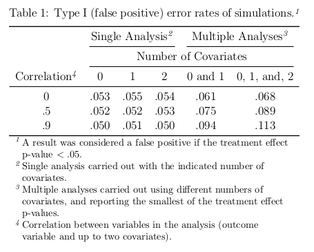