.row[ .col-7[ .title[ # Linear Regression ] .subtitle[ ## Simplest Machine Learning Algorithm to Start with ] .author[ ### Laxmikant Soni <br> [blog](https://laxmikants.github.io) <br> [<i class="fab fa-github"></i>](https://github.com/laxmiaknts) [<i class="fab fa-twitter"></i>](https://twitter.com/laxmikantsoni09) ] .affiliation[ ] ] .col-5[ .logo[ <img src="figures/rmarkdown.png" width="480" /> ] ] ] --- # Linear Regression .pull-left[ ## Definition * A linear equation that models a function such that if we give any `x` to it, it will predict a value `y` , where both `x and y` are input and output varaibles respectively. These are numerical and continous values. * It is the most simple and well known algorithm used in machine learning. ] -- .pull-right[ ## Flowchart 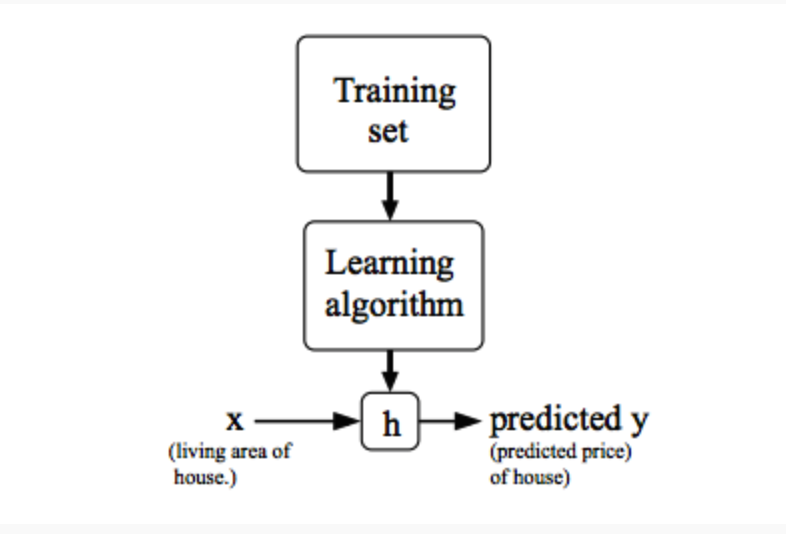<!-- --> * The above Flowchart represents that we choose our training set, feed it to an algorithm, it will learn the patterns and will output a function called `Hypothesis function 'H(x)'`. We then give any `x` value to that function and it will output an estimated `y` value for it. * For historical reasons, this function `H(x)` is called `hypothesis function.` <br> ] --- # Univariate Linear Regression .pull-left[ ## Definition * When you have one feature / variable `x` as an input to the function to predict `y`, we call this `Univariate Linear Regression` problem. <p align='center'>H(x) = θ₀ + θ₁x</p> Other way of representing this formula as what we are familiar with: <p align='center'>H(x) = b + mx</p> > Where : >- b = θ₀ 👉 y intercept >- m = θ₁ 👉 slope >- x = x 👉 feature / input variable ] -- .pull-right[ ## Model 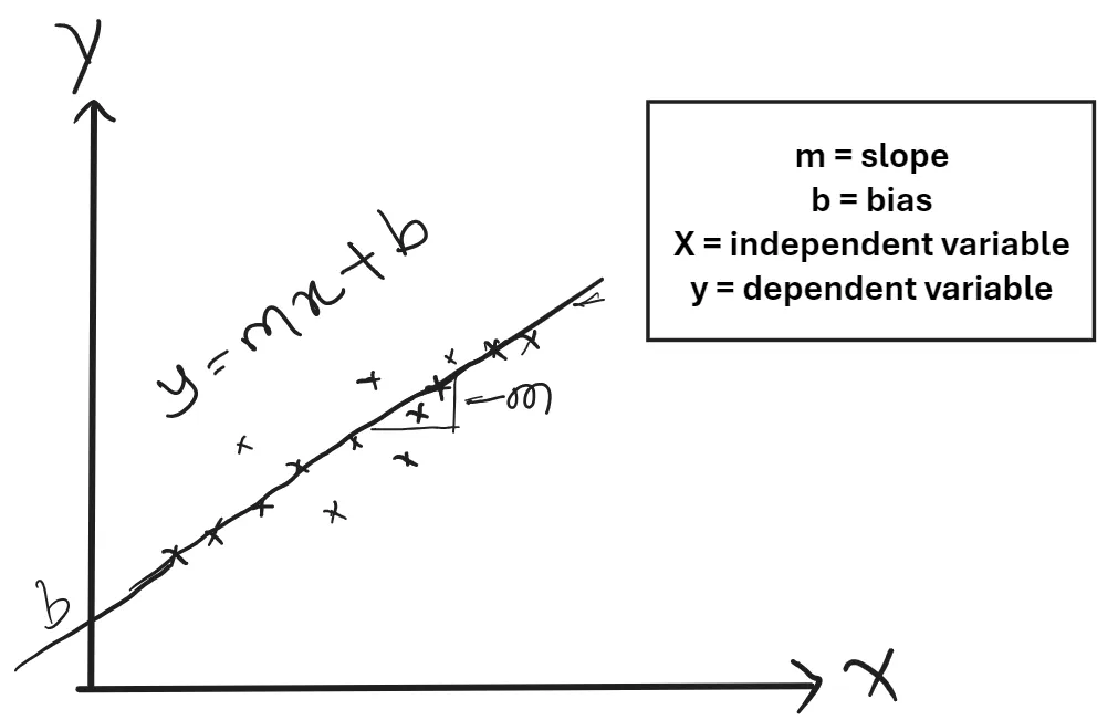<!-- --> ] --- # Cost Function .pull-left[ ## Definition - The **cost function** in univariate linear regression quantifies the difference between the model’s predictions and the actual data points. - Minimizing the cost function helps find the optimal parameters $$ \theta_0 \text{ and } \theta_1 $$ that best fit the data. ] -- .pull-right[ ## Formula for Cost Function - The cost function formula is given by: `$$J(\theta_0, \theta_1) = \frac{1}{2m} \sum_{i=1}^m \left( H(x^{(i)}) - y^{(i)} \right)^2$$` > Where : >- h(xⁱ) 👉 hypothesis function >- yⁱ 👉 actual values of `y` >- 1/m 👉 gives Mean of Squared Errors >- 1/2 👉 Mean is halved as a convenience for the computation of the `Gradient Descent`. This cost function is also called as `Squared Error Function` or `Mean Squared Error`. <br> ] --- # Gradient Descent .pull-left[ ## What is Gradient Descent? * how to "find the lowest point in a hilly landscape." * `gradient descent` is like rolling a marble down a hill: it will move in the direction of the `steepest slope` until it reaches the `lowest point`. ] -- .pull-right[ <!-- --> ] .pull-bottom[ *"The difference between simply rolling the marble down the hill and throwing it from a distance illustrates the concept of the `learning rate.`" ] --- # Gradient Descent - Learning Rate .pull-left[ ## What is Learning Rate? * The learning rate (α) is a hyperparameter that controls how much the model's parameters are adjusted during training with each iteration of the gradient descent algorithm. * A small learning rate (similar to rolling the marble): * Changes to the parameters are made slowly, allowing for more precise convergence to the minimum of the cost function. *A large learning rate (similar to throwing the marble): *Parameters are adjusted more significantly, which can lead to faster convergence in some cases. ] -- .pull-right[ <!-- --> ] --- # Gradient Descent for Univariate variable .pull-left[ ## Definition So now we have our hypothesis function and we have a way of measuring how well it fits into the data. Now we need to estimate the parameters in the hypothesis function. That's where `Gradient Descent` comes in.<br> `Gradient Descent` is used to minimize the cost function `J`, minimizing `J` is same as minimizing `MSE` to get best possible fit line to our data. ## Formula for Cost Function - The cost function formula is given by: `$$J(\theta_0, \theta_1) = \frac{1}{2m} \sum_{i=1}^m \left( H(x^{(i)}) - y^{(i)} \right)^2$$` ] -- .pull-right[ #### Formula for Gradient Descent $$ `\begin{aligned} \theta_0 &:= \theta_0 - \alpha \frac{\partial}{\partial \theta_0} J(\theta) \\ \theta_1 &:= \theta_1 - \alpha \frac{\partial}{\partial \theta_1} J(\theta) \end{aligned}` $$ > Where : >- `:=` 👉 Is the Assignment Operator >- `α` 👉 is `Alpha`, it's the number which is called learning rate. If its too high it may fail to converge and if too low then descending will be slow. >- 'θ_j' 👉 Taking Gradient Descent of a feature or a column of a dataset. > - ∂/(∂θ_j) J(θ₀,θ₁) 👉 Taking partial derivative of `MSE` cost function. <br> ] --- # Gradient Descent for Univariate variable .pull-top[ ## Visualization 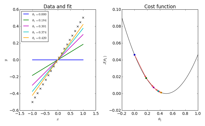<!-- --> ### Explanation of the Visualization: - The graph shows how the cost function decreases over iterations as the parameters are updated. - The arrows indicate the direction of the gradient, demonstrating how the parameters are adjusted towards the minimum cost. ] --- # Gradient Descent for Univariate variable .pull-top[ ### Steps of Gradient Descent: 1. **Initialize parameters**: Start with random values for `$$( \theta_0 , \theta_1 )$$`. 2. **Calculate the gradient**: Determine the gradient or derivative of the cost function with respect to each parameter. 3. **Update parameters**: Adjust the parameters using the learning rate `$$( \alpha ):$$` $$ \theta_j := \theta_j - \alpha \frac{\partial J(\theta_0, \theta_1)}{\partial \theta_j} $$ 4. **Repeat**: Continue the process until convergence (i.e., when the cost function stabilizes). ] --- # Gradient Descent for Univariate variable .pull-top[ **Now Let's apply Gradient Descend to minmize our `MSE` function.** <br> In order to apply `Gradient Descent`, we need to figure out the partial derivative term.<br> So let's solve partial derivative of cost function `J`. `$$\frac{\partial}{\partial \theta_0} J(\theta) = \frac{\partial}{\partial \theta_0} \left( \frac{1}{2m} \sum_{i=1}^{m} \left( (\theta_0 + \theta_1 x^{(i)}) - y^{(i)} \right)^2 \right)$$` `$$\frac{\partial}{\partial \theta_1} J(\theta) = \frac{\partial}{\partial \theta_1} \left( \frac{1}{2m} \sum_{i=1}^{m} \left( (\theta_0 + \theta_1 x^{(i)}) - y^{(i)} \right)^2 \right)$$` <br> ] --- # Gradient Descent for Univariate variable .pull-top[ Now let's plug these 2 values to our `Gradient Descent`: `$$\theta_0 := \theta_0 - \alpha \left( \frac{1}{m} \sum_{i=1}^{m} \left( (\theta_0 + \theta_1 x^{(i)}) - y^{(i)} \right) \right)$$` `$$\theta_1 := \theta_1 - \alpha \left( \frac{1}{m} \sum_{i=1}^{m} \left( (\theta_0 + \theta_1 x^{(i)}) - y^{(i)} \right) x^{(i)} \right)$$` <br> > **Note :** 🚩<br> > - Cost Function for Linear Regression is always going to be Convex or Bowl Shaped Function, so this function doesn't have any local minimum but one global minimum, thus always converging to global minimum. > - The above hypothesis function has 2 parameters, θ₀ & θ₁, so Gradient Descent will run on each feature, hence here two times, one for feature and one for base `(y-intercept)`, to get minimum value of `j`. So if we have `n` features, Gradient Descent will run on all `n+1` features. ] --- # Implementing Gradient Descent in Python .pull-left[ ## Importing necessary libraries ```python import numpy as np import matplotlib.pyplot as plt import pandas as pd ``` -- ] .pull-right[ * `numpy` is a powerful numerical library in Python, primarily used for handling arrays, numerical computations, and mathematical operations on data. * `matplotlib.pyplot` is a plotting library for creating static, animated, and interactive visualizations in Python. * `pandas` is a data analysis and manipulation library that provides data structures like DataFrames and Series for working with structured data. ] --- # Implementing Gradient Descent in Python .pull-left[ ## Generating sample data ```python # Generate synthetic data np.random.seed(0) # For reproducibility m = 100 # Number of data points X = 2.5 * np.random.rand(m, 1) # Size of the house (in thousands of square feet) y = 1.5 * X + np.random.randn(m, 1) * 0.5 # Price of the house (in thousands) ``` -- ] .pull-right[ * np.random.rand(m, 1) generates an array of shape (100, 1) with random values between 0 and 1. * Multiplying by 2.5 scales these values to be between 0 and 2.5. This represents the feature, which is the "size of the house" in thousands of square feet (e.g., 1.5 here would mean 1500 square feet). * So, X will contain 100 values for house sizes ranging from 0 to 2.5 thousand square feet. * Here, y is the target variable representing the "price of the house" (in thousands). * The term 1.5 * X represents a linear relationship where the price increases with the size, with a slope of 1.5 (indicating that, for each additional thousand square feet, the price increases by 1.5 thousand units). ] --- # Implementing Gradient Descent in Python .pull-left[ ## Define Cost function ```python def compute_cost(X, y, theta): m = len(y) predictions = X.dot(theta) cost = (1 / (2 * m)) * np.sum(np.square(predictions - y)) return cost ``` ] -- .pull-right[ * X: The feature matrix, where each row represents a training example (in this case, house sizes). * y: The actual target values (house prices) for each training example. * theta: The parameters (weights) of the model, which we'll adjust to minimize the cost. ] --- # Implementing Gradient Descent in Python .pull-left[ ## Define Gradient descent function ```python # Gradient descent function def gradient_descent(X, y, theta, alpha, iterations): m = len(y) cost_history = np.zeros(iterations) for i in range(iterations): predictions = X.dot(theta) errors = predictions - y theta -= (alpha / m) * (X.T.dot(errors)) cost_history[i] = compute_cost(X, y, theta) return theta, cost_history ``` ] -- .pull-right[ The gradient_descent function iteratively adjusts theta to minimize the cost function. In each iteration, it: * Predicts values using theta. * Computes the errors. * Updates theta in the direction that reduces the cost. * Records the cost in cost_history. The function returns the optimized parameters and a history of cost values across iterations, showing how the model learns over time. ] --- # Implementing Gradient Descent in Python .pull-left[ ## Prepare Data ```python # Prepare data X_b = np.c_[np.ones((m, 1)), X] theta_initial = np.random.randn(2, 1) # Hyperparameters alpha = 0.1 iterations = 1000 ``` ] -- .pull-right[ In summary, this setup prepares the feature matrix X to include an intercept, initializes theta randomly, and defines the learning rate and iteration count for gradient descent. ] --- # Implementing Gradient Descent in Python .pull-left[ ## Run Gradient Descent ```python # Run gradient descent theta_final, cost_history = gradient_descent(X_b, y, theta_initial, alpha, iterations) print(f"Final parameters (theta): {theta_final.ravel()}") ``` ``` ## Final parameters (theta): [0.11107554 1.487387 ] ``` ```python # Plot cost history plt.plot(range(iterations), cost_history, color='blue') plt.xlabel('Number of Iterations') plt.ylabel('Cost (J)') plt.title('Cost Function Convergence') plt.show() ``` ] -- .pull-right[ <!-- --> ] --- # Implementing Gradient Descent in Python .pull-left[ ## Plot Data and regression line ```python # Plot the data and the regression line plt.scatter(X, y, color='green', label='Data points') plt.plot(X, X_b.dot(theta_final), color='red', label='Regression line') plt.xlabel('Size of house (thousands of square feet)') plt.ylabel('Price of house (thousands)') plt.title('House Price Prediction') plt.legend() plt.show() ``` ] -- .pull-right[ <!-- --> ] --- class: inverse, center, middle # Thanks