In this section, we will discuss linear models with more than one predictors, i.e., multiple regression.
Multiple predictors
When you have an outcome variable and more than one predictor, you can fit a multiple regression. Let me do one on R with the data we used last time. This time, instead of predicting RT based on frequency alone, we predict it based on frequency and length.
This was easy - we just added Length as a predictor simply by typing “+ Length.” However, it is not obvious how coefficients and standard errors are calculated. The goal here is to understand what’s being done under the hood.
Before moving on, one thing you should realize is that now the effect of (log) frequency went away (in our sample). This is because length and frequency are correlated (if you calculate Pearson’s R, you get about -0.54).
Keep this observation in mind as we discuss how best-fitting coefficients are calculated.
Linear equations with multiple predictors
Recall that we had the following equation for a linear model with a single predictor:
\[
\hat{y_i} = b_0 + b_1x_i
\]
When we have more than one predictor (say two predictors), we can extend this equation by adding an additional slope term and multiply it by the second predictor variable (\(x_2\)).
\[
\hat{y_i} = b_0 + b_1x_{1i} + b_2x_{2i}
\]
Remember that to fit a linear model is to find coefficient values that minimizes the sum of residuals. In a regression with single predictor, calculating \(b_1\) by hand can be done relatively easily using the following equation we used last time.
To give you some intution, look at the numerator of the first equation (\(b_1\)). \(SS_{x_1y}\) expresses the covariance between \(x_1\) and \(y\) (technically covariance is calculated by dividing this value by (n-1), but this doesn’t matter in the current context because they will cancel out). This term is multiplied by the sum of squares for \(x_2\) (\(SS_{x_2x_2}\)), which expresses the amount of dispersion in \(x_2\). So the numerator in the first equation should be larger when \(x_1\) and \(y\) are strongly correlated and when \(x_2\) varies a lot.
Now, look to the right of the subtraction sign in the numerator of the first equation. \(SS_{x_2y}\) expresses the covariance between \(x_2\) and \(y\). This is multiplied by the covariance between \(x_1\) and \(x_2\). So the numerator would be smaller when \(x_2\) and \(y\) co-vary more strongly and \(x_1\) and \(x_2\) co-vary more strongly.
The important thing to note is that \(b_1\) reflects how strongly \(x_1\) and \(y\) co-vary but after taking into account how strongly \(x_1\) and \(x_2\) and \(x_2\) and \(y\) co-vary. This is why the effect of log frequency \(b_1\) got smaller (and non-significant): \(x_2\) and \(y\) are correlated and \(x_1\) (frequency) and \(x_2\) (length) are correlated.
These values matche with the coefficients the lm function spit out.
Matrix notation of linear equations
As we increase the number of predictors, calculating coefficients using equations like above becomes painful. Here I will introduce a matrix notation of the linear equation, which will be useful in understanding more complex models. Here’s the equation:
\[
\vec{y} = X\vec{b} + \vec{e}
\]
Throughout, I will use the arrow superscript to denote a n x 1 vector, and an uppercase letter to denote a m x n matrix.
If we have n observations and k number of predictors, \(X\) is a n x (k + 1) matrix and is known as design matrix, \(Y\) is a n x 1 column vector, \(b\) is a (k + 1) x 1 column vector, and \(e\) is a n x 1 column vector.
If you are not familiar with matrix algebra, these formula probably make no sense. I will try to unpack them. But before doing so, let’s go through the basics of linear algebra and work with the equation.
A crush course of matrix algebra
Matrix multiplication
Suppose that you want to multiply the following 2 x 3 matrix and 3 x 2 matrix.
First, consider the first row of the first matrix (2 6 3) and the first column of the second matrix (5 6 2) and calculate the sum of the element-wise products (called dot products). \(2 * 5 + 6 * 6 + 3 * 2 = 52\). This fills in the top-left cell of the resulting matrix (which has the number of rows of the first matrix and the number of columns of the second matrix).
Next, you calculate the sum of the element-wise product of the first row of the first matrix (2 6 3) and the second column of the second matrix (1 9 3). \(2*1 + 6*9 + 3*7 = 77\). This fills the top-middle cell of the resulting matrix.
\[
\begin{bmatrix}
2 & 6 & 3 \\
3 & 4 & 8 \\
\end{bmatrix}
\begin{bmatrix}
5 & 1 \\
6 & 9 \\
2 & 7 \\
\end{bmatrix} =
\begin{bmatrix}
52 & 77 \\
? & ? \\
\end{bmatrix}
\] You then fill the second row of the resulting matrix by element-wise multiply the second row of the first matrix and each column of the second matrix. You get:
In R, you can multiply a matrix using %*% operator. By the way, you can also transpose a matrix by using the funtion t().
A =matrix(c(2,3,6,4,3,8) , nrow =2, ncol =3)B =matrix(c(5,6,2,1,9,7), nrow =3, ncol =2)AB = A %*% BAB
     [,1] [,2]
[1,]   52   77
[2,]   55   95
t(AB)
     [,1] [,2]
[1,]   52   55
[2,]   77   95
Note that matrix multiplication is associative but notcommutative. Thus, \(A(BC) = (AB)C\), but \(AB ≠ BA\). Note also that matrix multiplication can only be done when the number of rows of the first matrix and the number of columns in the second matrix are the same.
Matrix transposition
The \('\) sign means that it’s a transposed matrix. If you transpose a m x n matrix, the resulting matrix is n x m matrix where the columns and rows are swapped. For instance, suppose you have a 3 x 2 matrix, \(A\).
It is helpful to know some of the rule of matrix transposition. Especially, take note of the last rule.
(A’ )’ = A
(A + B)’ = A’ + B’
(cA)’ = cA’
(AB)’ = B’A’
Matrix inverse
An inverse matrix of \(A\) is defined as a matrix that, when \(A\) is multiplied with it, result in an identity matrix. An identity matrix is a square matrix with all its diagonal elements equal to 1, and zeroes everywhere else. The number of columns and rows of an identity matrix is always the same. For example, the following matrices are all identity matrices.
If you multiply a matrix \(A\) with its inverse, \(A^{-1}\), you end up with an identity matrix.
\[
AA^{-1} =
\begin{bmatrix}
a & b \\
c & d \\
\end{bmatrix}
\begin{bmatrix}
a & b \\
c & d \\
\end{bmatrix}^{-1}
=
\begin{bmatrix}
1 & 0 \\
0 & 1 \\
\end{bmatrix}
\]
Figuring out what the inverse of a matrix can be messy. But here’s the formula for a 2 x 2 matrix.
\[
\begin{bmatrix}
a & b \\
c & d \\
\end{bmatrix}^{-1} = \frac{1}{ad-bc}
\begin{bmatrix}
d & -b \\
-c & a \\
\end{bmatrix}
\]
Only n x n matrices (i.e., square matrices) are invertible, though not all n x n matrices are invertible (non-invertible matrices are called singular).
In R, an inverse matrix can be computed by the solve() function.
This matches with the output of the lm function in R.
Standard errors
To calculate standard errors associated with coefficients, we first need to compute the residual sum of squares (RSS), which is just \(\sum e^2\) =\(\sum (y-Xb)^2\).
If you divide this by the degrees of freedom (n - k - 1), you get Mean Squared Error (MSE):
\[
MSE = \frac{RSS}{n-k-1}
\]
The variance associated with the \(j\)th coefficient can be computed by multiplying MSE with the $j$th diagonal element of the matrix \((X'X)^{-1}\) (this is known as precision matrix)
\[
Var(b_j) = MSE(X'X)^{-1}_{jj}
\]
If you take the square root of the variance, you get the standard error:
\[
SE(b_j) = \sqrt{Var(b_j)}
\]
Let’s compute the standard errors of coefficients and the p values in R. The degrees of freedom are n minus the number of parameters used to estimate the error (b0, b1, b2). In our case, 27.
pt(b1/SE_b1,27,lower.tail =TRUE)*2# lower.tail = TRUE when the coefficient is negative
[1] 0.5580113
pt(b2/SE_b2,27,lower.tail =FALSE)*2
[1] 0.002110237
But where does the coefficient formula come from?
To explain, I unfortunately need to first talk about derivatives, partial derivatives, and matrix differentiation.
Derivatives
Derivatives of a function express the rate of change of the output of the function, with respect to a certain argument variable. For example,
\[
f(x) = x^2
\]
Suppose that you pick two points, a and b, and define the difference from a to b as \(\Delta x\). For instance, if the point a is 5 and the point b is 6, \(\Delta x\) is 6-5 = 1.
With these two points, we can compute how much y changes when x changes by \(\Delta x\). f()
\[
\frac{f(\Delta x + x) - f(x)}{\Delta x}
\]
Now, we set \(\Delta x\) to be infinitesimally close to 0. This is the derivative of the function with respect to x, and expresses the rate of change in the function with respect to x.
\[
\frac{dy}{dx} = \lim_{\Delta x \rightarrow 0} \frac{f(\Delta x + x) - f(x)}{\Delta x}
\]
For example, if the function is \(f(x) = x^2\), you have
\[
\frac{dy}{dx} = \lim_{\Delta x \rightarrow 0} \frac{(\Delta x + x)^2 - x^2}{\Delta x}\\
= \frac{\Delta x^2 + 2\Delta x x + x^2 - x^2}{\Delta x}\\
= 2x
\]
In, you can figure out the derivative of a polynomial function \(f(x) = x^n\) by using the following formula
\[
\frac{d}{dx} x^n = nx^{(n-1)}
\]
Partial derivatives
Partial derivatives are computed when there are more than one argument variables. Partial derivatives express the rate of change of the output, with respect to one of the variable and when the other variables are treated as constant. For instance, suppose you have the following function.
\[
f(x,y) = x^2 + y^2
\]
The partial derivative of this function with respect to \(x\) is:
\[
\frac{\partial f(x,y)}{\partial x} = 2x
\]
The partial derivative of this function with respect to \(y\) is:
\[
\frac{\partial f(x,y)}{\partial y} = 2y
\]
These could be derived from the limit definition of derivatives.
\[
\frac{\partial f(x,y)}{\partial x} = \lim_{\Delta x \rightarrow 0} \frac{f(\Delta x + x, y) - f(x, y)}{\Delta x}
\]
Plugging in appropriate values:
\[
\frac{\partial f(x,y)}{\partial x} = \lim_{\Delta x \rightarrow 0} \frac{ (\Delta x + x)^2 + y^2 - (x^2 + y^2)}{\Delta x}\\
= \lim_{\Delta x \rightarrow 0} \frac{ \Delta x^2 + 2\Delta xx + x^2 + y^2 - x^2 - y^2}{\Delta x}\\
= \lim_{\Delta x \rightarrow 0} \Delta x + 2x\\
= 2x
\]
Derivatives of a function involving a matrix with respect to a vector
Here’s a cheat sheet for figuring out a derivative of a function involving matrix:
Suppose you have a function:
\[
f(x) = A\vec{x}
\]
where A is a 2 x 2 matrix and x is a 2 x 1 vector. Say we have the following.
\[
\begin{bmatrix}
a & b\\
c & d
\end{bmatrix}\begin{bmatrix}
x_1\\
x_2
\end{bmatrix}
\]
Here, a, b, c d are constants. Matrix multiplication yields:
\[
\begin{bmatrix}
ax_1 + b x_2 \\
c x_1 + dx_2
\end{bmatrix}
\]
This means that multiplication of 2 x 2 matrix and 2 x 1 vector can be expressed as involving two functions, each a vector as an argument:
\[
\begin{bmatrix}
f_1(x_1, x_2) = ax_1 + b x_2 \\
f_2(x_1, x_2) = c x_1 + dx_2
\end{bmatrix}
\]
Derivative a function involving a matrix with respect to a vector has the following definition (this matrix is known as the Jacobian matrix):
Finally, we have to know the derivatives of functions like the following:\[
f(\vec{x}) = \vec{x}' A \vec{x}
\]
The derivative of this function with respect to \(\vec{x}\) is \(2A\vec{x}\). Here’s the derivation. Suppose that we have the same matrix A and the vector \(\vec{x}\) like above:
\[
\begin{bmatrix}
x_1 & x_2
\end{bmatrix}
\begin{bmatrix}
a & b\\
c & c\\
\end{bmatrix}
\begin{bmatrix}
x_1\\
x_2
\end{bmatrix}
\]
If you multiply these, you get just a one function.
\[
ax_1^2 + bx_1x_2 + cx_1x_2 + dx_2^2
\]
We have two argument variables for this function. The derivative is:
For symmetric matrices (matrices where transposition makes no difference), the result can be written as \(2A\vec{x}\).
Deriving the formula for calculating best-fitting coefficients
Finally we can talk about where the formula came from. Recall that we had the following equation:
\[
\vec{y} = X\vec{b} + \vec{e}
\]
You can manipulate this equation to get:
\[
\vec{e} = \vec{y} - X\vec{b}
\]
To find the best-fitting coefficients is to minimize the squared sum of errors (\(\sum (e_i^2)\)). \(\sum e^2\) is actually the same thing as multiplying the error vector (\(\vec{e}\)) with the transposed version of it. Thus, the following holds:
We want to find out when the derivative is 0. Intuitively, when a derivative is 0, the rate of change (in this case, the rate of change in \(\sum (e_i^2)\) with respect to \(\vec{b}\)) is 0. For a reason I don’t go into, the least square error method always involve “convex” function (see the figure below). This means you can say that the error is minimized when the rate of change in the squared sum of errors with respect to coefficients is 0.
Thus, we want to solve the following equation:
\[
0 = 2\vec{y}'X - 2\vec{b}'X'X
\]
with algebra:
\[
\vec{b}'X'X = \vec{y}'X
\]
You can multiply both sides of the equation by \((X'X)^{-1}\), which eliminates X’X on the left side:
\[
\vec{b}' = \vec{y}'X(X'X)^{-1}
\]
Now, we can transpose both sides of the equation.
\[
\vec{b} = (\vec{y}'X(X'X)^{-1})'
\]
This is:
\[
\vec{b} = (X'X)^{-1}X'\vec{y}
\]
Source Code
---author: Shota Mommatitle: "Multiple Regression"format: html: code-tools: true code-folding: show---In this section, we will discuss linear models with more than one predictors, i.e., **multiple regression**.## Multiple predictorsWhen you have an outcome variable and more than one predictor, you can fit a **multiple regression**. Let me do one on R with the data we used last time. This time, instead of predicting RT based on frequency alone, we predict it based on frequency and length.```{r}suppressPackageStartupMessages(library("tidyverse"))df <-read_csv("/Users/shota/Documents/Teaching/Fall2024/Statistics/data/LexDec.csv", show_col_types =FALSE)df$logf <-log(df$Frequency)m <-lm(RT ~ logf + Length, data = df)summary(m)$coeff```This was easy - we just added Length as a predictor simply by typing "+ Length." However, it is not obvious how coefficients and standard errors are calculated. The goal here is to understand what's being done under the hood.Before moving on, one thing you should realize is that now the effect of (log) frequency went away (in our sample). This is because length and frequency are correlated (if you calculate Pearson's R, you get about -0.54).```{r}plot(df$logf, df$Length)abline(lm(df$logf ~ df$Length))```Keep this observation in mind as we discuss how best-fitting coefficients are calculated.## Linear equations with multiple predictorsRecall that we had the following equation for a linear model with a single predictor:$$\hat{y_i} = b_0 + b_1x_i$$\When we have more than one predictor (say two predictors), we can extend this equation by adding an additional slope term and multiply it by the second predictor variable ($x_2$).$$\hat{y_i} = b_0 + b_1x_{1i} + b_2x_{2i}$$Remember that to fit a linear model is to find coefficient values that minimizes the sum of residuals. In a regression with single predictor, calculating $b_1$ by hand can be done relatively easily using the following equation we used last time.$$b_1 = \frac{SS_{xy}}{SS_{xx}} = \frac{\sum_i^n({x_i - \bar{x}) (y_i - \bar{y}) }}{\sum_i^n(x_i - \bar{x})^2}$$$$b_0 = \bar{y_i} - b_1\bar{x_i}$$But when we have two predictors, we have three coefficients to figure out. Things already get... tedious.$$b_1 = \frac{SS_{x_1y}SS_{x_2x_2} - SS_{x_2y}SS_{x_1x_2}}{SS_{x_1x_1}SS_{x_2x_2} - SS_{x_1x_2}SS_{x_1x_2}} \\= \frac{\sum (x_{1i} - \bar{x_1})(y_i - \bar{y})\sum(x_{2i} - \bar{x_2})^2 - \sum(x_{2i} - \bar{x})(y_i - \bar{y_i})\sum(x_{1i} - \bar{x_1})(x_{2i} - \bar{x_2})}{\sum(x_{1i} - \bar{x_1})^2 \sum (x_{2i} -\bar{x_2})^2 - \sum(x_{1i} - \bar{x_1})(x_{2i} - \bar{x_2}) \sum(x_{1i} - \bar{x_1})(x_{2i} - \bar{x_2})}$$$$b_2 = \frac{SS_{x_2y}SS_{x_1x_1} - SS_{x_1y}SS_{x_1x_2}}{SS_{x_1x_1}SS_{x_2x_2} - SS_{x_1x_2}SS_{x_1x_2}} \\= \frac{\sum (x_{2i} - \bar{x_2})(y_i - \bar{y})\sum(x_{1i} - \bar{x_1})^2 - \sum(x_{1i} - \bar{x})(y_i - \bar{y_i})\sum(x_{1i} - \bar{x_1})(x_{2i} - \bar{x_2})}{\sum(x_{1i} - \bar{x_1})^2 \sum (x_{2i} -\bar{x_2})^2 - \sum(x_{1i} - \bar{x_1})(x_{2i} - \bar{x_2}) \sum(x_{1i} - \bar{x_1})(x_{2i} - \bar{x_2})}$$$$b_0 = \bar{y} - b_1\bar{x_1} - b_2\bar{x_2}$$To give you some intution, look at the numerator of the first equation ($b_1$). $SS_{x_1y}$ expresses the covariance between $x_1$ and $y$ (technically covariance is calculated by dividing this value by (n-1), but this doesn't matter in the current context because they will cancel out). This term is multiplied by the sum of squares for $x_2$ ($SS_{x_2x_2}$), which expresses the amount of dispersion in $x_2$. So the numerator in the first equation should be larger when $x_1$ and $y$ are strongly correlated and when $x_2$ varies a lot.Now, look to the right of the subtraction sign in the numerator of the first equation. $SS_{x_2y}$ expresses the covariance between $x_2$ and $y$. This is multiplied by the covariance between $x_1$ and $x_2$. So the numerator would be smaller when $x_2$ and $y$ co-vary more strongly and $x_1$ and $x_2$ co-vary more strongly.The important thing to note is that $b_1$ reflects how strongly $x_1$ and $y$ co-vary but after taking into account how strongly $x_1$ and $x_2$ and $x_2$ and $y$ co-vary. This is why the effect of log frequency $b_1$ got smaller (and non-significant): $x_2$ and $y$ are correlated and $x_1$ (frequency) and $x_2$ (length) are correlated.Let's verify if this formula works in R:```{r}SS_x1y <-sum((df$logf -mean(df$logf)) * (df$RT -mean(df$RT)))SS_x2y <-sum((df$Length -mean(df$Length)) * (df$RT -mean(df$RT)))SS_x1x1 <-sum((df$logf -mean(df$logf))^2)SS_x2x2 <-sum((df$Length -mean(df$Length))^2)SS_x1x2 <-sum((df$logf -mean(df$logf)) * (df$Length -mean(df$Length)))b1 = (SS_x1y*SS_x2x2 - SS_x2y*SS_x1x2)/(SS_x1x1*SS_x2x2 - SS_x1x2^2)b2 = (SS_x2y*SS_x1x1 - SS_x1y*SS_x1x2)/(SS_x1x1*SS_x2x2 - SS_x1x2^2)b1b2```Once we figure out the values of $b_1$ and \$b_2\$, calculating $b_0$ is easy:$$b_0 = \bar{y} - b_1\bar{x_1} - b_2\bar{x_2}$$```{r}b0 =mean(df$RT) - b1*mean(df$logf) - b2*mean(df$Length)b0```These values matche with the coefficients the lm function spit out.## Matrix notation of linear equationsAs we increase the number of predictors, calculating coefficients using equations like above becomes painful. Here I will introduce a matrix notation of the linear equation, which will be useful in understanding more complex models. Here's the equation:$$\vec{y} = X\vec{b} + \vec{e}$$Throughout, I will use the arrow superscript to denote a n x 1 vector, and an uppercase letter to denote a m x n matrix.If we have n observations and k number of predictors, $X$ is a n x (k + 1) matrix and is known as **design matrix**, $Y$ is a n x 1 column vector, $b$ is a (k + 1) x 1 column vector, and $e$ is a n x 1 column vector.If we have just one predictor:$$\begin{bmatrix}y_1 \\y_2 \\... \\y_n \\\end{bmatrix} =\begin{bmatrix}1 & x_1 \\1 & x_2 \\... & ... \\1 & x_n \\\end{bmatrix}\begin{bmatrix}b_0 \\b_1 \\\end{bmatrix} +\begin{bmatrix}e_0 \\e_1 \\... \\e_n \\\end{bmatrix}$$If we have two:$$\begin{bmatrix}y_1 \\y_2 \\... \\y_n \\\end{bmatrix} =\begin{bmatrix}1 & x_{11} & x_{12} \\1 & x_{21} & x_{22} \\... & ... \\1 & x_{n1} & x_{n2} \\\end{bmatrix}\begin{bmatrix}b_0 \\b_1 \\b_2\end{bmatrix} +\begin{bmatrix}e_0 \\e_1 \\... \\e_n \\\end{bmatrix}$$And so forth. How do we find best-fitting $\vec{b}$? Here's the equation for finding the best-fitting $b$.$$\vec{b} = \begin{bmatrix}b_0 \\b_1 \\... \\b_k \\\end{bmatrix} = (X'X)^{-1} X'\vec{y}$$If you are not familiar with matrix algebra, these formula probably make no sense. I will try to unpack them. But before doing so, let's go through the basics of linear algebra and work with the equation.## A crush course of matrix algebra### Matrix multiplicationSuppose that you want to multiply the following 2 x 3 matrix and 3 x 2 matrix.$$\begin{bmatrix}2 & 6 & 3 \\3 & 4 & 8 \\\end{bmatrix} \begin{bmatrix}5 & 1 \\6 & 9 \\2 & 7 \\\end{bmatrix}$$First, consider the first row of the first matrix (2 6 3) and the first column of the second matrix (5 6 2) and calculate the sum of the element-wise products (called **dot products**). $2 * 5 + 6 * 6 + 3 * 2 = 52$. This fills in the top-left cell of the resulting matrix (which has the number of rows of the first matrix and the number of columns of the second matrix).$$\begin{bmatrix}2 & 6 & 3 \\3 & 4 & 8 \\\end{bmatrix} \begin{bmatrix}5 & 1 \\6 & 9 \\2 & 7 \\\end{bmatrix} =\begin{bmatrix}52 & ? \\? & ? \\\end{bmatrix} $$Next, you calculate the sum of the element-wise product of the first row of the first matrix (2 6 3) and the second column of the second matrix (1 9 3). $2*1 + 6*9 + 3*7 = 77$. This fills the top-middle cell of the resulting matrix.$$\begin{bmatrix}2 & 6 & 3 \\3 & 4 & 8 \\\end{bmatrix} \begin{bmatrix}5 & 1 \\6 & 9 \\2 & 7 \\\end{bmatrix} =\begin{bmatrix}52 & 77 \\? & ? \\\end{bmatrix} $$ You then fill the second row of the resulting matrix by element-wise multiply the second row of the first matrix and each column of the second matrix. You get:$$\begin{bmatrix}2 & 6 & 3 \\3 & 4 & 8 \\\end{bmatrix} \begin{bmatrix}5 & 1 \\6 & 9 \\2 & 7 \\\end{bmatrix} =\begin{bmatrix}52 & 77 \\55 & 96 \\\end{bmatrix} $$In R, you can multiply a matrix using %\*% operator. By the way, you can also transpose a matrix by using the funtion t().```{r}A =matrix(c(2,3,6,4,3,8) , nrow =2, ncol =3)B =matrix(c(5,6,2,1,9,7), nrow =3, ncol =2)AB = A %*% BABt(AB)```Note that matrix multiplication is **associative** but *not* **commutative**. Thus, $A(BC) = (AB)C$, but $AB ≠ BA$. Note also that matrix multiplication can only be done when the number of rows of the first matrix and the number of columns in the second matrix are the same.### Matrix transpositionThe $'$ sign means that it's a transposed matrix. If you transpose a m x n matrix, the resulting matrix is n x m matrix where the columns and rows are swapped. For instance, suppose you have a 3 x 2 matrix, $A$.$$A = \begin{bmatrix}1 & 2 \\3 & 4 \\5 & 6 \\\end{bmatrix} $$The transposed version of $A$, $A'$, is just:$$A' = \begin{bmatrix}1 & 3 & 5 \\2 & 4 & 6 \\\end{bmatrix} $$It is helpful to know some of the rule of matrix transposition. Especially, take note of the last rule.- (A' )' = A- (A + B)' = A' + B'- (cA)' = cA'- (AB)' = B'A'### Matrix inverseAn inverse matrix of $A$ is defined as a matrix that, when $A$ is multiplied with it, result in an **identity matrix**. An identity matrix is a square matrix with all its diagonal elements equal to 1, and zeroes everywhere else. The number of columns and rows of an identity matrix is always the same. For example, the following matrices are all identity matrices.$$\begin{bmatrix}1 & 0 \\0 & 1 \\\end{bmatrix} \\\begin{bmatrix}1 & 0 & 0 \\0 & 1 & 0 \\0 & 0 & 1 \\\end{bmatrix} \\\begin{bmatrix}1 & 0 & 0 & 0 \\0 & 1 & 0 & 0 \\0 & 0 & 1 & 0 \\0 & 0 & 0 & 1 \\\end{bmatrix} $$If you multiply a matrix $A$ with its inverse, $A^{-1}$, you end up with an identity matrix.$$AA^{-1} =\begin{bmatrix}a & b \\c & d \\\end{bmatrix} \begin{bmatrix}a & b \\c & d \\\end{bmatrix}^{-1}= \begin{bmatrix}1 & 0 \\0 & 1 \\\end{bmatrix} $$Figuring out what the inverse of a matrix can be messy. But here's the formula for a 2 x 2 matrix.$$\begin{bmatrix}a & b \\c & d \\\end{bmatrix}^{-1} = \frac{1}{ad-bc}\begin{bmatrix}d & -b \\-c & a \\\end{bmatrix}$$Only n x n matrices (i.e., square matrices) are **invertible**, though not all n x n matrices are invertible (non-invertible matrices are called singular).In R, an inverse matrix can be computed by the solve() function.```{r}ABsolve(AB)AB %*%solve(AB)```### Calculating coefficientsNow we have all the tools necessary to solve the equation for figuring out best fitting coefficients:$$\vec{b} = \begin{bmatrix}b_0 \\b_1 \\... \\b_k \\\end{bmatrix} = (X'X)^{-1} X'\vec{y}$$```{r}Y =matrix(df$RT, ncol =1)X =matrix(c(rep(1,length(df$logf)), df$logf, df$Length), nrow =length(df$logf), ncol =3)B =solve((t(X) %*% X)) %*%t(X) %*%YB```This matches with the output of the lm function in R.## Standard errorsTo calculate standard errors associated with coefficients, we first need to compute the residual sum of squares (RSS), which is just $\sum e^2$ =$\sum (y-Xb)^2$.If you divide this by the degrees of freedom (n - k - 1), you get Mean Squared Error (MSE):$$MSE = \frac{RSS}{n-k-1}$$The variance associated with the $j$th coefficient can be computed by multiplying MSE with the \$j\$th diagonal element of the matrix $(X'X)^{-1}$ (this is known as **precision matrix**)$$Var(b_j) = MSE(X'X)^{-1}_{jj}$$If you take the square root of the variance, you get the standard error:$$SE(b_j) = \sqrt{Var(b_j)}$$Let's compute the standard errors of coefficients and the p values in R. The degrees of freedom are n minus the number of parameters used to estimate the error (b0, b1, b2). In our case, 27.```{r}y = df$RTn =length(y)k =2ones <-rep(1, n)X =matrix(c(ones, log(df$Frequency), df$Length) ,nrow = n, ncol = k+1)RSS =sum((y - (X %*% B))^2)MSE = RSS/(n - k -1)XX <-solve((t(X) %*%X))SE_b0 =sqrt(MSE*XX[1,1])SE_b1 =sqrt(MSE*XX[2,2])SE_b2 =sqrt(MSE*XX[3,3])SE_b0SE_b1SE_b2pt(b0/SE_b0,27,lower.tail =FALSE)*2pt(b1/SE_b1,27,lower.tail =TRUE)*2# lower.tail = TRUE when the coefficient is negativept(b2/SE_b2,27,lower.tail =FALSE)*2```## But where does the coefficient formula come from?To explain, I unfortunately need to first talk about **derivatives, partial derivatives**, and **matrix differentiation**.### DerivativesDerivatives of a function express the rate of change of the output of the function, with respect to a certain argument variable. For example,$$f(x) = x^2$$Suppose that you pick two points, a and b, and define the difference from a to b as $\Delta x$. For instance, if the point a is 5 and the point b is 6, $\Delta x$ is 6-5 = 1.With these two points, we can compute how much y changes when x changes by $\Delta x$. f()$$\frac{f(\Delta x + x) - f(x)}{\Delta x}$$Now, we set $\Delta x$ to be infinitesimally close to 0. This is the derivative of the function with respect to x, and expresses the rate of change in the function with respect to x.$$\frac{dy}{dx} = \lim_{\Delta x \rightarrow 0} \frac{f(\Delta x + x) - f(x)}{\Delta x}$$For example, if the function is $f(x) = x^2$, you have$$\frac{dy}{dx} = \lim_{\Delta x \rightarrow 0} \frac{(\Delta x + x)^2 - x^2}{\Delta x}\\= \frac{\Delta x^2 + 2\Delta x x + x^2 - x^2}{\Delta x}\\= 2x$$In, you can figure out the derivative of a polynomial function $f(x) = x^n$ by using the following formula$$\frac{d}{dx} x^n = nx^{(n-1)} $$### Partial derivativesPartial derivatives are computed when there are more than one argument variables. Partial derivatives express the rate of change of the output, with respect to one of the variable and when the other variables are treated as constant. For instance, suppose you have the following function.$$f(x,y) = x^2 + y^2$$The partial derivative of this function with respect to $x$ is:$$\frac{\partial f(x,y)}{\partial x} = 2x$$The partial derivative of this function with respect to $y$ is:$$\frac{\partial f(x,y)}{\partial y} = 2y$$These could be derived from the limit definition of derivatives.$$\frac{\partial f(x,y)}{\partial x} = \lim_{\Delta x \rightarrow 0} \frac{f(\Delta x + x, y) - f(x, y)}{\Delta x}$$Plugging in appropriate values:$$\frac{\partial f(x,y)}{\partial x} = \lim_{\Delta x \rightarrow 0} \frac{ (\Delta x + x)^2 + y^2 - (x^2 + y^2)}{\Delta x}\\= \lim_{\Delta x \rightarrow 0} \frac{ \Delta x^2 + 2\Delta xx + x^2 + y^2 - x^2 - y^2}{\Delta x}\\= \lim_{\Delta x \rightarrow 0} \Delta x + 2x\\= 2x$$### Derivatives of a function involving a matrix with respect to a vectorHere's a cheat sheet for figuring out a derivative of a function involving matrix:Suppose you have a function:$$f(x) = A\vec{x}$$where A is a 2 x 2 matrix and x is a 2 x 1 vector. Say we have the following.$$\begin{bmatrix}a & b\\c & d\end{bmatrix}\begin{bmatrix}x_1\\x_2\end{bmatrix}$$Here, a, b, c d are constants. Matrix multiplication yields:$$\begin{bmatrix}ax_1 + b x_2 \\c x_1 + dx_2\end{bmatrix}$$This means that multiplication of 2 x 2 matrix and 2 x 1 vector can be expressed as involving two functions, each a vector as an argument:$$\begin{bmatrix}f_1(x_1, x_2) = ax_1 + b x_2 \\f_2(x_1, x_2) = c x_1 + dx_2\end{bmatrix}$$Derivative a function involving a matrix with respect to a vector has the following definition (this matrix is known as the **Jacobian** matrix):$$\frac{\partial f(x)}{\partial x} = \begin{bmatrix}\frac{\partial f_1}{\partial x_1} & \frac{\partial f_1}{\partial x_2} \\\frac{\partial f_2}{\partial x_1} & \frac{\partial f_2}{\partial x_2} \\\end{bmatrix}$$If you do the partial differentiation in each cell, you end up with a matrix you started out with.$$\frac{\partial}{\partial \vec{x}} A \vec{x} = \begin{bmatrix}a & b \\c & d \\\end{bmatrix}$$This is the matrix A we started with. Thus, the derivative of a function involving a matrix f(x) = Ax with respect to the vector x is:$$\frac{\partial}{\partial \vec{x}} A\vec{x} = A\$$Finally, we have to know the derivatives of functions like the following:$$f(\vec{x}) = \vec{x}' A \vec{x}$$The derivative of this function with respect to $\vec{x}$ is $2A\vec{x}$. Here's the derivation. Suppose that we have the same matrix A and the vector $\vec{x}$ like above:$$\begin{bmatrix}x_1 & x_2\end{bmatrix}\begin{bmatrix}a & b\\c & c\\\end{bmatrix}\begin{bmatrix}x_1\\x_2\end{bmatrix}$$If you multiply these, you get just a one function.$$ax_1^2 + bx_1x_2 + cx_1x_2 + dx_2^2$$We have two argument variables for this function. The derivative is:$$\frac{\partial}{\partial x} \vec{x}'A\vec{x} =\begin{bmatrix}\frac{\partial f}{\partial x_1}\\\frac{\partial f}{\partial x_2}\end{bmatrix}\\= \begin{bmatrix}2ax_1 + bx_2 + cx_2 \\bx_1 + cx_1 + 2dx_2\end{bmatrix}$$This matrix can be derived from:$$\begin{bmatrix}2ax_1 + bx_2 + cx_2 \\bx_1 + cx_1 + 2dx_2\end{bmatrix} = A\vec{x} + A'\vec{x}$$ For symmetric matrices (matrices where transposition makes no difference), the result can be written as $2A\vec{x}$.### Deriving the formula for calculating best-fitting coefficientsFinally we can talk about where the formula came from. Recall that we had the following equation:$$\vec{y} = X\vec{b} + \vec{e}$$You can manipulate this equation to get:$$\vec{e} = \vec{y} - X\vec{b}$$To find the best-fitting coefficients is to minimize the squared sum of errors ($\sum (e_i^2)$). $\sum e^2$ is actually the same thing as multiplying the error vector ($\vec{e}$) with the transposed version of it. Thus, the following holds:$$\sum (e_i^2) = \vec{e}'\vec{e}\\= (\vec{y} - X\vec{b})'(\vec{y} - X\vec{b}) \\=(\vec{y}' - \vec{b}'X') (\vec{y} - X\vec{b})\\=\vec{y}'\vec{y} - \vec{y}'X\vec{b}-\vec{b}'X'\vec{y} + \vec{b}'X'X\vec{b}$$You can think of the squared sum of errors as an output of the function that takes the coefficient vector ($\vec{b}$) as an argument:$$f(\vec{b}) = \vec{y}'\vec{y} - \vec{y}'X\vec{b}-\vec{b}'X'\vec{y} + \vec{b}'X'X\vec{b}$$In this context, $\vec{y}'X\vec{b}$ and $\vec{b}'X'\vec{y}$ are actually the same:```{r}t(Y) %*% X %*% Bt(B) %*%t(X) %*% Y```So,$$f(\vec{b}) = \vec{y}'\vec{y} - 2\vec{y}'X\vec{b} + \vec{b}'X'X\vec{b}$$The derivative of this function with respect to $\vec{b}$ is (note that X'X is always symmetric):$$\frac{\partial f(\vec{b})}{\partial \vec{b}} =-2\vec{y}'X + 2\vec{b}'X'X$$We want to find out when the derivative is 0. Intuitively, when a derivative is 0, the rate of change (in this case, the rate of change in $\sum (e_i^2)$ with respect to $\vec{b}$) is 0. For a reason I don't go into, the least square error method always involve "convex" function (see the figure below). This means you can say that the error is minimized when the rate of change in the squared sum of errors with respect to coefficients is 0.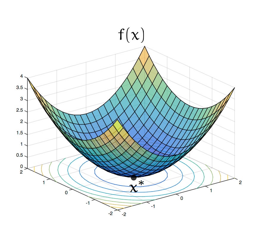{width="265"}Thus, we want to solve the following equation:$$0 = 2\vec{y}'X - 2\vec{b}'X'X$$with algebra:$$\vec{b}'X'X = \vec{y}'X$$You can multiply both sides of the equation by $(X'X)^{-1}$, which eliminates X'X on the left side:$$\vec{b}' = \vec{y}'X(X'X)^{-1}$$Now, we can transpose both sides of the equation.$$\vec{b} = (\vec{y}'X(X'X)^{-1})'$$This is:$$\vec{b} = (X'X)^{-1}X'\vec{y}$$

