Despite my penchant for coding constantly in R, I'm primarily a biochemistry student. Today I'm going to hit two birds with one stone by using R to create a diagram for my notes (which are themselves written in \( \LaTeX \)).
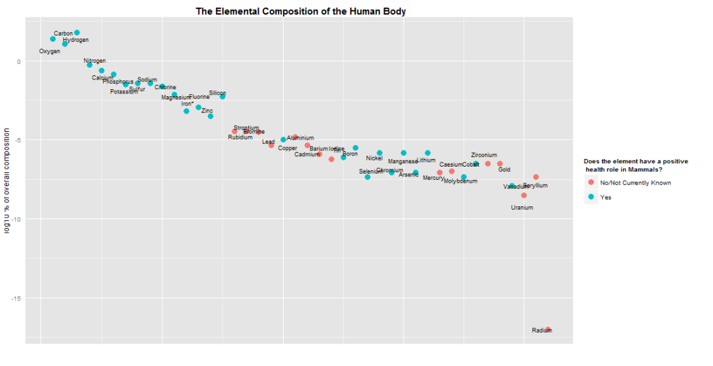
The diagram shows the chemical composition (percentage atoms) of the human body. Besides the more common elements (\( C, H, O, N, P \)) there are also a myriad of elements with specialised but essential roles in the body. Selenium - a sulpherlike element often found in wretched smelling compounds - is present in the oft-ignored 21st amino-acid[1] selenocysteine, which as a constituent of the enzyme deiodinase helps regulate the metabolic rate. Cobalt is the workhorse of cofactor B12, which acts as a free-radical generator in order to rearrange a certain fat breakdown product. Despite cobalt's minute concentration \( (1:10^{6}) \), a B12-deficiency[2] usually proves fatal within three years.
Some of the elements that are labelled as not having a positive health effect do play some role in human metabolism - for example rubidium is treated much like the \( K^{+} \) (pottasium) ion, and lead is a powerful inhibitor of some blood-forming[3] enzymes. As per the legend title, these are not considered as having a positive health effect; their absence from the body is not missed.
I used the readHTMLTable function in the XML package to get the data, which was taken from Wikipedia. Wikipedia has a wide range of well formatted tables, particularly for statistics by country. In this case, the statistics are slightly anomalous: the proportions sum to slightly over 1. My guess is that either the page authors, or myself, fudged one of the numbers by an order of magnitude. Maybe silicon; I'm surprised that so much silicon is present in human body (notwithstanding the obvious implant-jokes).
The HTML table is parsed in a reasonably workable format, with only one value that needs manual tweaking. The downside to this method of importing tables is that the resulting object has poorly-named components; X$NULL$Positive health role in mammals[7] looks more like ASCII art than legitimate R code.
suppressPackageStartupMessages(library(ggplot2))
suppressPackageStartupMessages(library(stringr))
suppressPackageStartupMessages(library(parallel))
suppressPackageStartupMessages(library(XML))

l <- base::length

rawHuman <- readHTMLTable(
    "http://en.wikipedia.org/wiki/Composition_of_the_human_body",
    as.data.frame = FALSE

)[2]
I'm trying to cut down on my use of the imperative programming paradigm; in my opinion the step-wise approach to programming leads to long, complex programs. These can usually be re-factored to use lambda expressions, parallel versions of the apply function, and one liners. The performance boost is just a bonus.
The elementPlot function takes the \( log_{10} \) of the composition percentage by element, adds a point to the plot, and draws a label near this point. By near, I mean that a random amount is added the position of the point (x, y), slightly randomising the label positions. I generated the graphic eight or nine times to get an overlap-free image. A genetic algorithm or calculus-heavy optimisation function would be neater, but would take much longer to write.[4]
The graphic is also colour coded: blue means that the element is biologically beneficial in mammals, and red means it is not. The raw Wikipedia data was not organised by a similarly simple TRUE/FALSE scheme. Instead, it provided a Yes/No value, sometimes followed by an explanation. I used the str_match function to try match the word “Yes” in the data; if it occurred the element was coloured blue, otherwise it was coloured red.
atomicPercent <- rawHuman$`NULL`$`Atomic percent`
atomicPercent <- atomicPercent[ind <- which(atomicPercent != "")]
atomicPercent[l(atomicPercent)] <- 1e-17

elementPlot <- function() {
    ggplot(data = data.frame(index = 1:l(atomicPercent), element = rawHuman$`NULL`$Element[ind],
        atomicPercent = as.numeric(atomicPercent), healthRole = unlist(mclapply(X = (role <- rawHuman$`NULL`$`Positive health role in mammals[7]`)[ind],
            FUN = function(x) {

                if (is.na(unlist(str_match(x, "Yes")))) {
                  "No/Not Currently Known"
                } else {
                  "Yes"
                }

            })))) + geom_point(aes(x = index, y = log10(atomicPercent), colour = healthRole),
        size = 4) + xlab("") + ylab("log10 % of overall composition") + geom_text(aes(x = index +
        sample((-5:5)/10, , size = l(atomicPercent), replace = TRUE), y = log10(atomicPercent) +
        sample((-7:7)/10, size = l(atomicPercent), replace = TRUE), label = element),
        size = 3.3) + opts(title = "The Elemental Composition of the Human Body",
        plot.title = theme_text(size = 15, face = "bold"), axis.line = theme_blank(),
        axis.ticks = theme_blank(), axis.text.x = theme_blank()) + scale_colour_discrete(name = "Does the element have a positive \n health role in Mammals?")
}
[1] The pedant in me must add the qualifier that selenocysteine is the 21st mammalian proteogenic amino acid
[2] Brought on by pernicious anaemia, which hinders the absorbsion of Vitamin B12 from the diet
[3] Enzymes involved in heme-synthesis, to be specific.
[4] Sorry about the unreadable ggplot2 code; R markdown ignores my common-lisp like indentation style by deleting whitespace. In this case it halfed the length of the block of code, doubling unreadability