Activity06 - Multinomial Logistic Regression
The Data
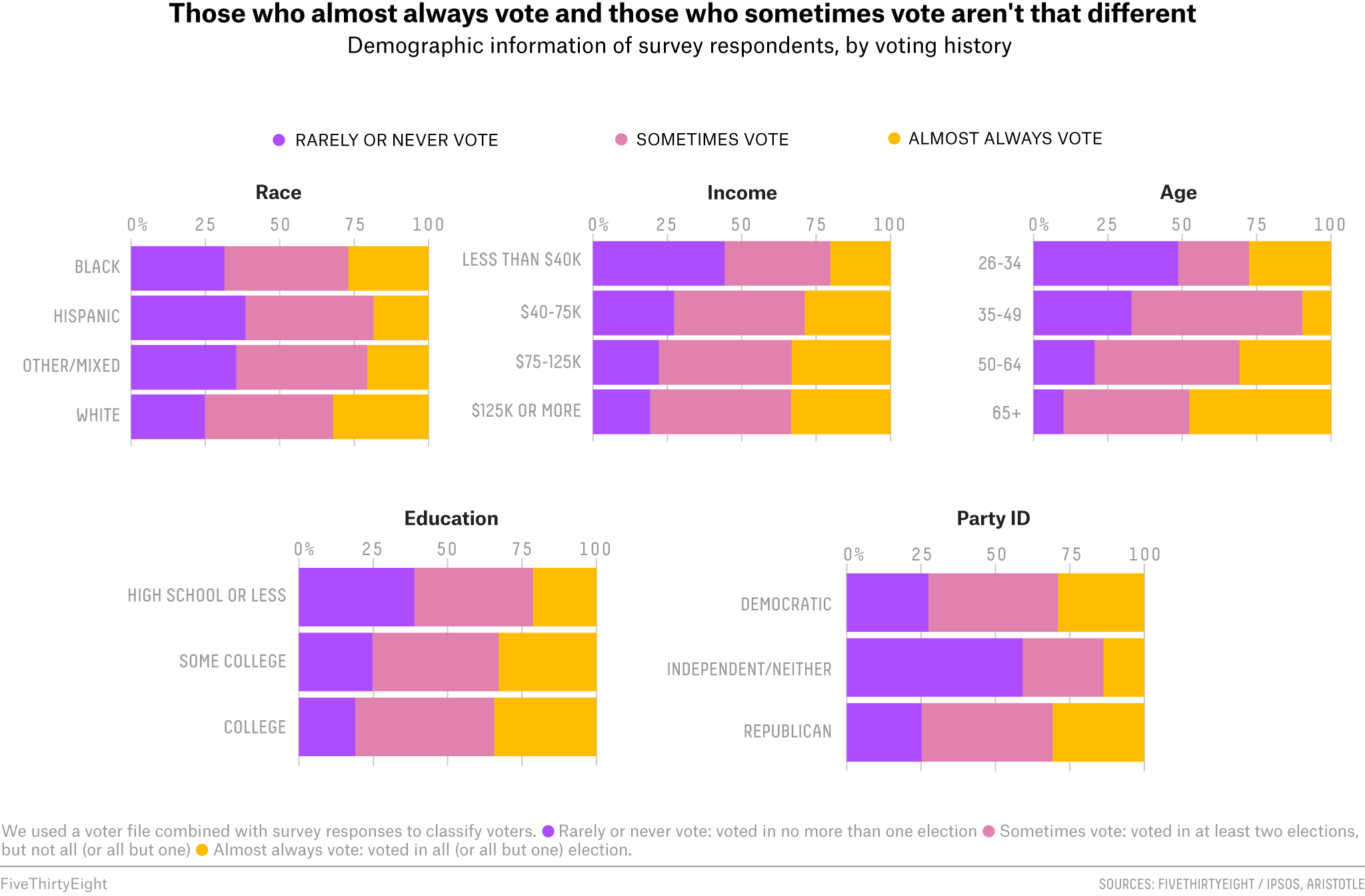
Today we will analyze data from an online Ipsos (a consulting firm)
survey that was conducted for a \(\texttt{FiveThirthyEight}\) article Why
Many Americans Don’t Vote.
You can read more about the survey design and respondents in the
README of their GitHub
repo for the data.
Briefly, respondents were asked a variety of questions about their
political beliefs, thoughts on multiple issues, and voting
behavior.
We will focus on the demographic variables and the respondent’s party
identification to understand whether a person is a probable voter (with
levels always, sporadic, rarely/never).
The specific variables we will use are (definitions are from the nonvoters_codebook.pdf):
ppage: Age of respondenteduc: Highest educational attainment categoryrace: Race of respondent, census categories Note: all categories except Hispanic are non-Hispanicgender: Gender of respondentincome_cat: Household income category of respondentQ30: Response to the question “Generally speaking, do you think of yourself as a…”- 1: Republican
- 2: Democrat
- 3: Independent
- 4: Another party, please specify
- 5: No preference
- -1: No response
voter_category: past voting behavior:- always: respondent voted in all or all-but-one of the elections they were eligible in
- sporadic: respondent voted in at least two, but fewer than all-but-one of the elections they were eligible in
- rarely/never: respondent voted in 0 or 1 of the elections they were eligible in
These data were originally downloaded from:
https://github.com/fivethirtyeight/data/tree/master/non-voters
Notes:
- Similarly to the data we used for the logistic regression portion of
this activity, the researchers have the variable labeled
gender, but it is unclear how this question was asked or what categorizations (if any) were provided to respondents to select from. We will use this as, “individuals that chose to provide their gender.” - The authors use weighting to make the final sample more representative on the US population for their article. We will not use weighting in this activity, so we will treat the sample as a convenience sample rather than a random sample of the population.
Load necessary packages
## ── Attaching core tidyverse packages ──────────────────────── tidyverse 2.0.0 ──
## ✔ dplyr     1.1.4     ✔ readr     2.1.5
## ✔ forcats   1.0.0     ✔ stringr   1.5.1
## ✔ lubridate 1.9.3     ✔ tibble    3.2.1
## ✔ purrr     1.0.2     ✔ tidyr     1.3.1
## ── Conflicts ────────────────────────────────────────── tidyverse_conflicts() ──
## ✖ dplyr::filter() masks stats::filter()
## ✖ dplyr::lag()    masks stats::lag()
## ℹ Use the conflicted package (<http://conflicted.r-lib.org/>) to force all conflicts to become errors## ── Attaching packages ────────────────────────────────────── tidymodels 1.2.0 ──
## ✔ broom 1.0.6 ✔ rsample 1.2.1
## ✔ dials 1.2.1 ✔ tune 1.2.1
## ✔ infer 1.0.7 ✔ workflows 1.1.4
## ✔ modeldata 1.3.0 ✔ workflowsets 1.1.0
## ✔ parsnip 1.2.1 ✔ yardstick 1.3.1
## ✔ recipes 1.0.10
## ── Conflicts ───────────────────────────────────────── tidymodels_conflicts() ──
## ✖ scales::discard() masks purrr::discard()
## ✖ dplyr::filter() masks stats::filter()
## ✖ recipes::fixed() masks stringr::fixed()
## ✖ dplyr::lag() masks stats::lag()
## ✖ yardstick::spec() masks readr::spec()
## ✖ recipes::step() masks stats::step()
## • Dig deeper into tidy modeling with R at https://www.tmwr.orgLoad the data
## Rows: 5836 Columns: 119
## ── Column specification ────────────────────────────────────────────────────────
## Delimiter: ","
## chr   (5): educ, race, gender, income_cat, voter_category
## dbl (114): RespId, weight, Q1, Q2_1, Q2_2, Q2_3, Q2_4, Q2_5, Q2_6, Q2_7, Q2_...
##
## ℹ Use `spec()` to retrieve the full column specification for this data.
## ℹ Specify the column types or set `show_col_types = FALSE` to quiet this message.
Select only required variables
# Select the required variables
nonvoters <- nonvoters %>%
  select(ppage, educ, race, gender, income_cat, Q30, voter_category)

#head(nonvoters)
glimpse(nonvoters)
## Rows: 5,836
## Columns: 7
## $ ppage <dbl> 73, 90, 53, 58, 81, 61, 80, 68, 70, 83, 43, 42, 48, 52,…
## $ educ <chr> "College", "College", "College", "Some college", "High …
## $ race <chr> "White", "White", "White", "Black", "White", "White", "…
## $ gender <chr> "Female", "Female", "Male", "Female", "Male", "Female",…
## $ income_cat <chr> "$75-125k", "$125k or more", "$125k or more", "$40-75k"…
## $ Q30 <dbl> 2, 3, 2, 2, 1, 5, 1, 2, 1, 3, 1, 2, 1, 5, 1, 1, 2, 1, 5…
## $ voter_category <chr> "always", "always", "sporadic", "sporadic", "always", "…After doing this, we will answer the following questions:
- Why did the authors chose to only include data from people who were eligible to vote for at least four election cycles?
Establishing Voting Patterns: By focusing on individuals who have been eligible to vote in multiple election cycles, the authors can more accurately assess long-term voting behavior. This helps in distinguishing between those who consistently vote, those who vote sporadically, and those who rarely or never vote.
Focus on Experienced Voters: Individuals who have been eligible for fewer election cycles might still be forming their voting habits. By including only those eligible for multiple cycles, the study can focus on voters with established behaviors, providing clearer insights into what influences consistent versus sporadic or non-voting behavior.
Impact of Long-Term Factors: Long-term eligibility allows the study to consider the impact of stable, long-term factors (like age, education, and income) on voting behavior, rather than short-term influences that might affect new voters.
- In the FiveThirtyEight article, the authors include visualizations
of the relationship between the voter
category and demographic variables. Let’s select two of these
demographic variables. Then, for each variable, we will create and
interpret a plot to describe its relationship with
voter_category.
Relationship Between Voter Category and Education
# Visualization for education
ggplot(nonvoters, aes(y = educ, fill = voter_category)) +
  geom_bar(position = "fill") +
  scale_x_continuous(labels = scales::percent) +
  labs(
    title = "Voter Category Distribution by Education",
    y = "Education Level",
    x = "Education",
    fill = "Voter Category"
  ) +
  theme_minimal()
Relationship Between Voter Category and Race
# Visualization for race
ggplot(nonvoters, aes(y = race, fill = voter_category)) +
  geom_bar(position = "fill") +
  scale_x_continuous(labels = scales::percent) +
  labs(
    title = "Voter Category Distribution by Race",
    y = "Race",
    x = "Race",
    fill = "Voter Category"
  ) +
  theme_minimal()
We need to do some data preparation before we fit our multinomial logistic regression model.
- We will address the following items:
- The variable
Q30contains the respondent’s political party identification.
Let’s create a new variable calledpartyin the dataset that simplifiesQ30into four categories: “Democrat”, “Republican”, “Independent”, “Other” (“Other” should also include respondents who did not answer the question).
- The variable
voter_categoryidentifies the respondent’s past voter behavior. Let’s convert this to a factor variable and ensure (hint: explorerelevel) that the “rarely/never” level is the baseline level, followed by “sporadic”, then “always”.
- The variable
# Select the required variables
nonvoters <- nonvoters %>%
  select(ppage, educ, race, gender, income_cat, Q30, voter_category)

# Create the new 'party' variable
nonvoters <- nonvoters %>%
  mutate(party = case_when(
    Q30 == 1 ~ "Republican",
    Q30 == 2 ~ "Democrat",
    Q30 == 3 ~ "Independent",
    Q30 == 4 | Q30 == 5 | Q30 == -1 ~ "Other"
  ))

# Convert voter_category to factor and set the baseline level
nonvoters <- nonvoters %>%
  mutate(voter_category = factor(voter_category, levels = c("rarely/never", "sporadic", "always")))
# Check the changes by creating a stacked bar graph
ggplot(nonvoters, aes(y = party, fill = voter_category)) +
geom_bar(position = "fill") +
scale_x_continuous(labels = scales::percent) +
labs(
title = "Voter Category Distribution by Party",
y = "",
x = "Party",
fill = "Voter Category"
) +
#scale_fill_manual(values = c("#ff5a5f", "#00a699", "#fc642d")) + # Using similar colors to FiveThirtyEight
theme_minimal()
Fitting the model
Previously, we have explored logistic regression where the
outcome/response/independent variable has two levels (e.g., “has
feature” and “does not have feature”).
We then used the logistic regression model
\[ \begin{equation*} \log\left(\frac{\hat{p}}{1-\hat{p}}\right) = \hat\beta_0 + \hat\beta_1x_1 + \hat\beta_2x_2 + \cdots + \hat\beta_px_p \end{equation*} \]
Another way to think about this model is if we are interested in
comparing our “has feature” category to the baseline “does not
have feature” category.
If we let \(y = 0\) represent the
baseline category, such that \(P(y_i
= 1 | X's) = \hat{p}_i1\) and \(P(y_i = 0 | X's) = 1 - \hat{p}_{i1} =
\hat{p}_{i0}\), then the above equation can be rewritten as:
\[ \begin{equation*} \log\left(\frac{\hat{p}_{i1}}{\hat{p}_{i0}}\right) = \hat\beta_0 + \hat\beta_1x_{i1} + \hat\beta_2x_{i2} + \cdots + \hat\beta_px_{ip} \end{equation*} \]
Recall that:
- The slopes (\(\hat\beta_p\))
represent when \(x_p\) increases by one
(\(x_p\)) unit, the odds of \(y = 1\) compared to the baseline \(y = 0\) are expected to multiply by a
factor of \(e^{\hat\beta_p}\).
-The intercept (\(\hat\beta0\)) represents when all \(x_j = 0\) (for \(j = 1, \ldots, p\)), the predicted odds of \(y = 1\) versus the baseline \(y = 0\) are \(e^{\hat\beta_0}\).
For a multinomial (i.e., more than two categories, say, labeled \(k = 1, 2, \ldots, K\)) outcome variable, \(P(y = 1) = p_1, P(y = 2) = p_2, \ldots, P(y = K) = p_k\), such that
\[ \begin{equation*} \sum_{k = 1}^K p_k = 1 \end{equation*} \]
This is called the multinomial distribution.
For a multinomial logistic regression model it is helpful to identify
a baseline category (say, \(y =
1\)).
We then fit a model such that \(P(y = k) =
p_k\) is a model of the \(x\)’s.
\[ \begin{equation*} \log\left(\frac{\hat{p}_{ik}}{\hat{p}_{i1}}\right) = \hat\beta_{0k} + \hat\beta_{1k}x_{i1} + \hat\beta_{2k}x_{i2} + \cdots + \hat\beta_{pk}x_{ip} \end{equation*} \]
Notice that for a multinomial logistic model, we will have separate
equations for each category of the outcome variable relative to
the baseline category.
If the outcome has \(K\) possible
categories, there will be \(K - 1\)
equations as part of the multinomial logistic model.
Suppose we have an outcome variable \(y\) with three possible levels coded as “A”, “B”, “C”. If “A” is the baseline category, then
\[ \begin{equation*} \begin{aligned} \log\left(\frac{\hat{p}_{iB}}{\hat{p}_{iA}}\right) &= \hat\beta_{0B} + \hat\beta_{1B}x_{i1} + \hat\beta_{2B}x_{i2} + \cdots + \hat\beta_{pB}x_{ip} \\ \log\left(\frac{\hat{p}_{iC}}{\hat{p}_{iA}}\right) &= \hat\beta_{0C} + \hat\beta_{1C}x_{i1} + \hat\beta_{2C}x_{i2} + \cdots + \hat\beta_{pC}x_{ip} \\ \end{aligned} \end{equation*} \]
Now we will fit a model using age, race, gender, income, and
education to predict voter category.
This is using {tidymodels}.
# Abbreviated recipe from previous activities
multi_mod <- multinom_reg() %>%
  set_engine("nnet") %>%
  fit(voter_category ~ ppage + educ + race + gender + income_cat, data = nonvoters)

multi_mod <- repair_call(multi_mod, data = nonvoters)

tidy(multi_mod) %>%
  print(n = Inf) # This will display all rows of the tibble
## # A tibble: 22 × 6
## y.level term estimate std.error statistic p.value
## <chr> <chr> <dbl> <dbl> <dbl> <dbl>
## 1 sporadic (Intercept) -0.887 0.167 -5.32 1.03e- 7
## 2 sporadic ppage 0.0476 0.00229 20.8 5.05e- 96
## 3 sporadic educHigh school or less -0.922 0.0957 -9.64 5.42e- 22
## 4 sporadic educSome college -0.357 0.0938 -3.81 1.40e- 4
## 5 sporadic raceHispanic -0.00655 0.126 -0.0521 9.58e- 1
## 6 sporadic raceOther/Mixed -0.373 0.157 -2.38 1.74e- 2
## 7 sporadic raceWhite -0.127 0.102 -1.25 2.10e- 1
## 8 sporadic genderMale -0.0961 0.0707 -1.36 1.74e- 1
## 9 sporadic income_cat$40-75k -0.127 0.110 -1.15 2.48e- 1
## 10 sporadic income_cat$75-125k -0.000882 0.106 -0.00832 9.93e- 1
## 11 sporadic income_catLess than $40k -0.663 0.112 -5.91 3.43e- 9
## 12 always (Intercept) -1.85 0.185 -10.0 1.18e- 23
## 13 always ppage 0.0606 0.00252 24.0 2.29e-127
## 14 always educHigh school or less -1.35 0.107 -12.7 7.65e- 37
## 15 always educSome college -0.412 0.100 -4.10 4.13e- 5
## 16 always raceHispanic -0.417 0.147 -2.84 4.46e- 3
## 17 always raceOther/Mixed -0.683 0.182 -3.74 1.82e- 4
## 18 always raceWhite 0.0392 0.111 0.353 7.24e- 1
## 19 always genderMale -0.211 0.0779 -2.70 6.83e- 3
## 20 always income_cat$40-75k -0.0669 0.120 -0.559 5.76e- 1
## 21 always income_cat$75-125k 0.147 0.113 1.29 1.95e- 1
## 22 always income_catLess than $40k -0.756 0.125 -6.05 1.43e- 9{tidymodels} is designed for cross-validation and so
there needs to be some “trickery” when we build models using the entire
dataset.
For example, when we type multi_mod$fit$call in our
Console, we should see the following output:
> multi_mod$fit$call
nnet::multinom(formula = voter_category ~ ppage + educ + race + gender + income_cat, data = data, trace = FALSE)
The issue here is data = data and should be
data = nonvoters. To repair this, we add the
following to our previous R code chunk and re-run it:
multi_mod <- repair_call(multi_mod, data = nonvoters)Then type multi_mod$fit$call in our
Console, we should see the following output:
> multi_mod$fit$call
nnet::multinom(formula = voter_category ~ ppage + educ + race + gender + income_cat, data = nonvoters, trace = FALSE)
Now, recall that the baseline category for the model is
"rarely/never".
Using our tidy(multi_mod) %>% print(n = Inf) output,
let’s complete the following items:
- Write the model equation for the log-odds of a person that the
“rarely/never” votes vs “always” votes.
That is, finish this equation using the estimated parameters:
\[ \begin{equation*} \log\left(\frac{\hat{p}_{\texttt{"always"}}}{\hat{p}_{\texttt{"rarely/never"}}}\right) = -1.854 + 0.061 \times \texttt{ppage} - 1.353 \times \texttt{educHigh school or less} - 0.412 \times \texttt{educSome college} \\ - 0.417 \times \texttt{raceHispanic} - 0.683 \times \texttt{raceOther/Mixed} - 0.211 \times \texttt{genderMale} - 0.756 \times \texttt{income\_catLess than \$40k} \end{equation*} \]
- For the equation in (3), interpret the slope for
genderMalein both log-odds and odds.
The coefficient for genderMale is -0.211.
Log-Odds Interpretation: Holding all other variables constant, being male (genderMale) decreases the log-odds of being in the “always” voter category compared to the “rarely/never” category by 0.211 units. In other words, males are less likely to be in the “always” voter category compared to females.
Odds = 𝑒log-odds
Odds Interpretation: For each unit increase in the genderMale variable (which is coded as 1 for male, 0 otherwise), the odds of being in the “always” voter category versus the “rarely/never” category change by a factor of 𝑒−0.211 (0.809)
Therefore, males have approximately 0.809 times the odds of being in the “always” voter category compared to females, holding all other variables constant.
This interpretation gives us insights into how gender influences the likelihood of being a consistent voter compared to rarely or never voting, adjusted for other demographic factors included in the model.
Note: The interpretation for the slope for
ppage is a little more difficult to interpret.
However, we could mean-center age (i.e., subtract the mean age from each
age value) to have a more meaningful interpretation.
Predicting
We could use this model to calculate probabilities.
Generally, for categories \(2, \ldots,
K\), the probability that the \(i^{th}\) observation is in the \(k^{th}\) category is,
\[ \begin{equation*} \hat{p}_{ik} = \frac{e^{\hat\beta_{0j} + \hat\beta_{1j}x_{i1} + \hat\beta_{2j}x_{i2} + \cdots + \hat\beta_{pj}x_{ip}}}{1 + \sum_{k = 2}^Ke^{\hat\beta_{0k} + \hat\beta_{1k}x_{1i} + \hat\beta_{2k}x_{2i} + \cdots + \hat\beta_{pk}x_{pi}}} \end{equation*} \]
And the baseline category, \(k = 1\),
\[ \begin{equation*} \hat{p}_{i1} = 1 - \sum_{k = 2}^K \hat{p}_{ik} \end{equation*} \]
However, we will let R do these calculations.
## # A tibble: 5,836 × 12
##    .pred_class `.pred_rarely/never` .pred_sporadic .pred_always ppage educ
##    <fct>                      <dbl>          <dbl>        <dbl> <dbl> <chr>
##  1 always                    0.0352          0.411        0.554    73 College
##  2 always                    0.0153          0.402        0.583    90 College
##  3 sporadic                  0.119           0.489        0.391    53 College
##  4 sporadic                  0.121           0.485        0.394    58 Some coll…
##  5 sporadic                  0.0930          0.505        0.402    81 High scho…
##  6 sporadic                  0.204           0.472        0.324    61 High scho…
##  7 sporadic                  0.0778          0.504        0.418    80 High scho…
##  8 sporadic                  0.102           0.515        0.382    68 Some coll…
##  9 sporadic                  0.0516          0.475        0.474    70 College
## 10 always                    0.0380          0.454        0.508    83 Some coll…
## # ℹ 5,826 more rows
## # ℹ 6 more variables: race <chr>, gender <chr>, income_cat <chr>, Q30 <dbl>,
## # voter_category <fct>, party <chr>## # A tibble: 5,836 × 4
## .pred_class `.pred_rarely/never` .pred_sporadic .pred_always
## <fct> <dbl> <dbl> <dbl>
## 1 always 0.0352 0.411 0.554
## 2 always 0.0153 0.402 0.583
## 3 sporadic 0.119 0.489 0.391
## 4 sporadic 0.121 0.485 0.394
## 5 sporadic 0.0930 0.505 0.402
## 6 sporadic 0.204 0.472 0.324
## 7 sporadic 0.0778 0.504 0.418
## 8 sporadic 0.102 0.515 0.382
## 9 sporadic 0.0516 0.475 0.474
## 10 always 0.0380 0.454 0.508
## # ℹ 5,826 more rowsHere we can see all of the predicted probabilities.
This is still rather difficult to view so a confusion
matrix can help us summarize how well the predictions fit the actual
values.
voter_conf_mat <- voter_aug %>%
  count(voter_category, .pred_class, .drop = FALSE)

voter_conf_mat %>%
  pivot_wider(
    names_from = .pred_class,
    values_from = n
  )
## # A tibble: 3 × 4
## voter_category `rarely/never` sporadic always
## <fct> <int> <int> <int>
## 1 rarely/never 586 815 50
## 2 sporadic 271 1994 309
## 3 always 243 1150 418We can also visualize how well these predictions fit the original values.
#voters %>%
voter_conf_mat |>
  ggplot(aes(x = voter_category)) +
  geom_bar() +
  labs(
    main = "Self-reported voter category"
    )
voter_conf_mat %>%
  ggplot(aes(x = voter_category, y = n, fill = .pred_class)) +
  geom_bar(stat = "identity") +
  labs(
    main = "Predicted vs self-reported voter category"
    )