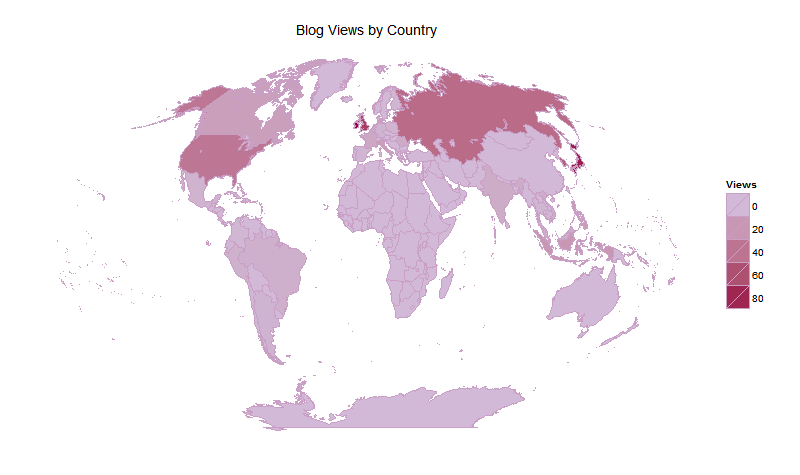
After months of being irked by the lack of decent projections in the mapproj package I decided to implement one of my own. There's no point having a function without data to use it on, so I made a map of the views by country of my Wordpress views, specifically for my graphic design blog. The data shows the views by country from February 25th 2012 to August 14th of the same year.
The results are a little surprising; a large percentage of my views come from Japan, Korea, and other countries in the East. My best explanation is that some of my graphic design projects involved modelling country-specific military equipment.
To get the WordPress data I simply copied the text and tidied it up manually - it was not long enough to justify using Regular Expression.
viewsByCountry <- data.frame(Ireland = 90, Japan = 83, United_Kingdom = 68,
    Republic_of_Korea = 52, Russian_Federation = 45, United_States = 38, Indonesia = 20,
    Philippines = 17, Italy = 15, Canada = 15, France = 10, Romania = 9, India = 8,
    Vietnam = 7, Malaysia = 7, Brazil = 6, Peru = 5, Netherlands = 5, Mexico = 4,
    Poland = 4, Argentina = 3, Germany = 3, Finland = 2, Spain = 2, Thailand = 2,
    Colombia = 1, Ecuador = 1, Cambodia = 1, Belgium = 1, Chile = 1)
To construct the choropleth each country is filled with a colour - which is dependant on the number of blog views from that country. That does present the problem of making sure the country actually existed at the time the maps package was constructed; political borders change frequently. We can check this using R's extraordinarily useful set theory operations.
suppressPackageStartupMessages(library(ggplot2))
mapsNames <- unique(unname(unlist(map_data("world")["region"])))
dataNames <- names(viewsByCountry)
setdiff(x = dataNames, y = mapsNames)
## [1] "United_Kingdom"     "Republic_of_Korea"  "Russian_Federation"
## [4] "United_States"
Now I have the names of the countries that don't appear in the maps package. It seems that when the map data was created the USSR still existed; I'm going to assign the views from the Russian Federation to the USSR region, at risk of offending half of Europe.
names(viewsByCountry)[names(viewsByCountry) == "United_Kingdom"] <- "UK"
names(viewsByCountry)[names(viewsByCountry) == "United_States"] <- "USA"
names(viewsByCountry)[names(viewsByCountry) == "Republic_of_Korea"] <- "South Korea"
names(viewsByCountry)[names(viewsByCountry) == "Russian_Federation"] <- "USSR"
The WordPress statistics are now ready to be viewed as a choropleth. Before I do that, I'm going to implement the Kavraisky VII projection.
The Kavraisky VII has a very simple definition; I could implement it in four lines. However, that would exclude fool-proofing and would make the code unamenable to extension. Instead I'm going to write a wrapper function which can hold as many map projections as I can implement. Each map projection gets its own function, with a name of the form ProjectKavraisky, ProjectGall and so on. These functions are called from within the Project wrapper function, depending on the map projection used (say “project” one more time…). This is done using function and argument matching.
The match.fun function lets you call a function with a function name variable. Here's a simple example:
f <- function(x){x}
g <- function(x){x+1}

name1 <- "f"
name2 <- "g"

match.fun(name1)(2)
match.fun(name2)(2)
Using function matching can be useful in a variety of circumstances, the most obvious is using a function on data, with the function used dependant on the data. In this case, the data is the argument for the parameter projection.
It's not quite flexible enough for my purposes. The case I provides contains two function, both of which have one argument x. What if each function requires different arguments. When I need to match both functions and parameters I like to use eval(parse()), a combination of functions that let you evaluate a string as code.
x = 1
y = 1

f <- function(x){x}
g <- function(x,y){(x*y)+1}

a1 <- "x"
a2 <- "x, y"

name1 <- "f"
name2 <- "g"

eval(
    parse(
        text = paste("match.fun(name1)(", a1, ")")
    )
)

eval(
    parse(
        text = paste("match.fun(name2)(", a2, ")")
    )
)
The strings (the text argument), when evaluated, become the following R code
match.fun(name1)( x )
match.fun(name2)( x, y )
Which reduces to
f(x)
g(x, y)
This is my favourite way of dynamically calling functions, which I included in my code below. It doesn't really need to be present, since I'm only including one projection (The Kavraisky VII), but it does make the code very extendible. Anyway, back to making the map.
The project wrapper function tests that the inputs are valid, removes invalid longitude/latitude coordinates, and matches the inputs to the appropriate function. It needs a few tweaks to the “projections” and “arguments” list to support other map projection functions, but its pretty flexible.
Project <- function(x = NULL, y = NULL, projection = "Kavraisky",
    remove = FALSE) {

    l <- base::length

    # add a few more projections, maybe Winkel-Tripel and Hammer-Wagner...

    projections <- list("Kavraisky")

    # the arguments to match to the function, using eval(parse())

    arguments <- list(Kavraisky = "x, y")

    # check that the inputs are numberical vectors, with x[i] el (-180:180),
    # y[i] el (-90:90)

    if (is.null(x) || is.null(y))
        stop("longitude(x) or latitude(y) missing")
    if (l(x) != l(y))
        stop("the longitude(x) and latitude(y) lengths differ")
    if (!(is.vector(x) && is.vector(y)))
        stop("the longitudes and latitudes must be supplied as vectors")
    if (!(is.numeric(x) && is.numeric(y)))
        stop("both the latitudes and longitudes must be numeric vectors")
    if (!is.element(projection, unlist(projections)))
        stop("valid map projection not included")

    if (remove) {

        if ((max(x) > 180 || max(y) > 90 || min(x) < -180 || min(x) < -90)) {

            validPairs <- intersect(intersect(which(x <= 180), which(x >= -180)),
                intersect(which(y <= 90), which(y >= -90)))

            if (l(validPairs) == 0)
                stop(paste("all longitude and latitude values are invalid - ensure some values meet the following:",
                  "latitudes[i] element (180, -179, ..., +180),", "latitudes[i] element (-90, -89, ..., +90)"))

            warning("some values are not valid latitude/longitude coordinates; excluding invalid coordinate pairs")

            x <- x[validPairs]
            y <- y[validPairs]

        }


    }

    # match the projection function based on the projection being used.  match
    # the arguments from the list 'arguments', evaluate the code with
    # eval(parse())

    funToCall <- paste("Project", projection, sep = "")
    matchedArguments <- arguments[[projection]]

    return(eval(parse(text = paste("match.fun(funToCall)(", matchedArguments,
        ")"))))

}


ProjectKavraisky <- function(x, y) {

    x = x * pi/180
    y = y * pi/180

    return(list(x = (3 * x)/(2 * pi) * ((pi^2)/(3) - abs(y)^2), y = y))

}
This block of code converts the views into a format that can be merged with the projected map data.
l <- base::length

data <- Project(unname(unlist(map_data("world")["long"])), unname(unlist(map_data("world")["lat"])),
    remove = FALSE)

mapData <- map_data("world")
mapData["long"] <- data$x
mapData["lat"] <- data$y

rm(data)

region = unname(unlist(mapData["region"]))
views = rep(0, l(region))

for (i in 1:l(region)) {

    if (is.element(region[i], names(viewsByCountry)))
        views[i] <- viewsByCountry[region[i]]

}
Finally, I add the number of views to the map data and plot the choropleth using ggplot2. The bulk of the code involves turning off guide lines and axes, and is identical to the code I used to visualise the trace-route paths to the Top 100 websites from my laptop.
mapData["Views"] <- unlist(views)

newPlot <- ggplot(legend = FALSE) + geom_polygon(data = mapData,
    aes(x = long, y = lat, group = group, fill = Views), colour = "#C99FC5") +
    opts(plot.background = theme_rect(fill = "white"), panel.background = theme_blank(),
        panel.border = theme_blank(), panel.grid.major = theme_blank(), panel.grid.minor = theme_blank(),
        axis.line = theme_blank(), axis.ticks = theme_blank(), axis.text.x = theme_blank(),
        axis.text.y = theme_blank(), axis.title.x = theme_blank(), axis.title.y = theme_blank(),
        title = "Blog Views by Country") + scale_fill_gradient(low = "#D1BAD7",
    high = "#950042")