• Hypothesis testing is an inferential procedure that uses sample data to evaluate the credibility of a hypothesis about a population.

• In hypothesis testing, you’re observing if a statement has either any significance or none.

• This significance is measured by a quantity called a p-value.

• The p-value (p) quantifies how well data supports your hypothesis.

• A p-value is set by a continuous range between 0 and 1.

• The significance determined by a p-value is determined by observing if p ≤ α (alpha; critical level)

• If the p-value is under the alpha, then that means our results our significant and we are “rejecting the null hypothesis”.

• Otherwise, we are accepting the null hypothesis and the results are not significant.

1. First you define your null hypothesis (H0; stating no relationship/significance) and the alternative hypothesis (H1; stating there is a relationship)

2. Select an alpha (significance level). It’s most common for you to see the alpha set as 0.05 (5%), but in other cases it’s usually 0.01 (1%)

3. Run a hypothesis test, this choice is dependent on what you feel meets your needs (Ex: T-test, Z-test, chi-squares, etc).

4. Then you calculate the p-value. I will show an example in a further slide.

5. Finally you will draw your conclusion based on the placing of the p-value relative to the alpha.

Scenario: You want to find out if there’s a significant differences between the averages of Group A vs. Group B on how they did on the ACTs.

Identification: - Null Hypothesis: Our averages are insignificantly different. We can quantify this by checking if the mean score of Group A is equal to that of Group B’s - Alternative Hypothesis: Our averages are significantly different, meaning both means are not equal to each other.

Significance Level: 0.05

Data: Group A:

##             variable value
## 1               Mean    85
## 2 Standard Deviation    10
## 3        Sample Size    30

Group B:

##             variable value
## 1               Mean    80
## 2 Standard Deviation    12
## 3        Sample Size    30

The formula for a z-score is: \[ z = \frac{X - μ}{σ} \]

z = z-score X = sample mean μ = population mean σ = standard deviation of the population

\[ z = \frac{{85 - 80}}{{\sqrt{\frac{{10^2}}{{30}} + \frac{{12^2}}{{30}}}}} \\ \sqrt{\frac{{10^2}}{{30}} + \frac{{12^2}}{{30}}} \approx 2.3094 \\ z = \frac{5}{2.3094} = 2.165 \]

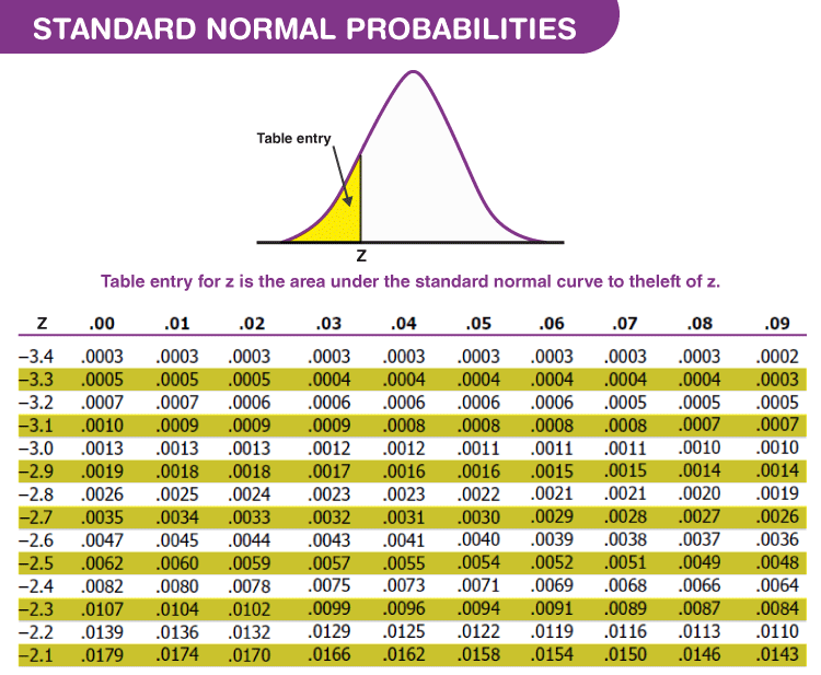
After getting the z-score, you will be able to find the p-value by using a standard normal table.

After using the chart, we decided that the p-value is 0.0304 which is less than the alpha. Meaning by conventional criteria, the test scores between both groups is statistically significant. This concludes our hypothesis testing.

Let’s start graphing the data to see what patterns we can pick up.

##  [1]  98.93754  69.41537  79.24349  78.14533  73.93402  94.33778  70.99800
##  [8]  94.11160  87.61459  66.36038  76.75967  85.88192  82.21481  97.40090
## [15]  82.82602  82.22904  97.16645  96.35078  77.87221  81.25548  96.25139
## [22] 108.73570  86.18728  86.08911  78.67039  71.14077  87.91473  92.84816
## [29]  97.59982  63.09095

##  [1]  84.75714  92.10595  92.81248  81.70091  89.96267  78.97040  73.73070
##  [8]  76.68855  97.40317  79.52888  87.27778  86.46511  96.90905  84.15114
## [15]  87.73997  74.78971  86.47543  80.59801  70.68183  90.04508  94.32401
## [22]  76.99337  53.36498  51.48786 112.19130  92.69430  82.81758  93.55406
## [29]  81.98741  74.61303

plot_ly() %>%
  add_histogram( x = ~groupA, name = 'Group A', opacity = 0.4) %>%
  add_histogram( x = ~groupB, name = 'Group B', opacity = 0.4) %>%
  layout(title = "Histogram of both Testing Groups",
         xaxis = list(title = "Value"),
         yaxis = list(title = "Frequency"),
         barmode = 'overlay')