This and other labs in this course are based on those initially developed by C.J. Gabbe and Iris Stewart Frey
epsg code and
proj4string definitionCreate a ‘Module5_Lab’ folder. Create a new RScript and save to your
‘Module5_Lab’ folder. Install the lwgeom package. Load the
packages we’re going to use today and set your working directory:
library(sf)
library(tidyverse)
library(tmap)
library(lwgeom)
library(units)

setwd("/Users/johndialesandro/Google Drive/My Drive/ENVS 117/04_Labs/Module5_Lab/")Download the fire hazard shapefile for state responsibility areas in Santa Cruz County you will need to scroll down .
We need to plot a quick map like we did lab 4. Notice we will get an Error: “Shape contains invalid polygons. Please fix it or set tmap_options(check.and.fix = TRUE) and rerun the plot” to fix this you can run sf_use_S2(FALSE) whihc will fix this issue
SRA_SC <- st_read("fhszs06_3_44.shp")
summary(SRA_SC)
sf_use_s2(FALSE)
qtm(SRA_SC, fill = "HAZ_CLASS", check.and.fix = TRUE)
Fix the order of the fire severity polygons like we did in Lab 4. The code is in the lab 4 document and also late on in this lab. Download and unzip the shapefile with all mobile home parks in California (these are data I cleaned previously).
MHPs_CA <- st_read("MHPs_HCD_022818_CLEAN.shp")
summary(MHPs_CA)

qtm(MHPs_CA)We’ll first check for an epsg (projection) code; if the
data don’t have an epsg code, we’ll need to project them
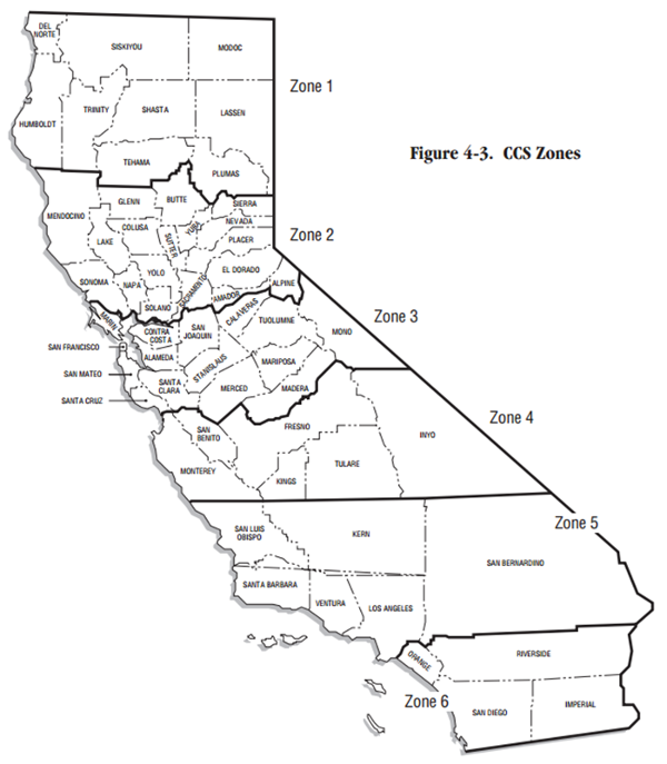
into California State Plane Zone 3. Remember this
map?
SRA_SC # check projection
SRA_SC <- st_transform(SRA_SC, crs = 2227) # project to California State Plane Zone 3
We’ll then do the same thing for the mobile home parks data.
MHPs_CA # check projection
MHPs_CA <- st_transform(MHPs_CA, crs = 2227) # project to California State Plane Zone 3epsg code and
proj4string definitionWhat is the epsg code for California State Plane zone 5?
Zone 3? Hint: use Google or Spatialreference.org.
What is the ‘proj4string’ definition for California State Plane zone 5? Zone 3? Hint: use Spatialreference.org. proj4string is being phased out, but you’ll still come across it periodically so it’s useful to understand.
Before we get too much farther, let’s clean up our data a bit. For
the fire hazard data, let’s just select the columns we want to keep. You
can use names to get a list of column names and
numbers.
names(SRA_SC)

SRA_SC <- select(SRA_SC, 1:3)
We also need to reorder the factors (like we did previously)
SRA_SC$HAZ_CLASS <- ordered(SRA_SC$HAZ_CLASS, levels = c("Moderate", "High", "Very High"))

SRA_SC$HAZ_CLASS # This will let you check the levels to make sure it worked
Our mobile home parks data includes all of the data in the state, so let’s filter it down to only the MHPs in Tuolumne County.
MHPs_SC <- filter(MHPs_CA, Conty_Nm == "SANTA CRUZ")Let’s add a field where we calculate the area of the fire hazard
zones in square feet (remember that the st_area
calculations will be based on the units of the CRS/projected coordinate
system).
SRA_SC$AreaSqFt <- st_area(SRA_SC)Now let’s add another column that converts square feet to acres (43,560 square feet = 1 acre)
SRA_SC$AreaAcres <- SRA_SC$AreaSqFt / 43560Here’s a way that you could calculate the area in acres in one step! Can you explain in plain language what this code is doing?
SRA_SC <- mutate(SRA_SC, AreaAcres2 = (st_area(SRA_SC)/43560)) # This is creating a second acres variable so you can compare AreaAcres and AreaAcres2.Regardless of the way that you create this variable – and in R there are usually at least several ways you can do achieve something – you’ll notice that the units listed next to the variable in the table aren’t correct. I generally encourage you to track the units of measure in the variable name, which will help someone if you export the data to different software.
You can either convert the units to the correct measure or you can drop the units attribute in the table:
# check the units
units(SRA_SC$AreaSqFt)
units(SRA_SC$AreaAcres) # check the units

# option 1: set units
SRA_SC$AreaSqFt <- set_units(SRA_SC$AreaSqFt, ft^2)
SRA_SC$AreaAcres <- set_units(SRA_SC$AreaAcres, acre)

# option 2: remove the units attribute altogether using base::as.numeric or units::drop_units
SRA_SC$AreaSqFt <- as.numeric(SRA_SC$AreaSqFt)
SRA_SC$AreaAcres <- as.numeric(SRA_SC$AreaAcres)Centroids allow us to identify the geographic center of each feature. This can be helpful for identifying the mean location within each feature or it can be part of a strategy for combining two datasets.
SRA_SC_cntrd <- st_centroid(SRA_SC)We can create buffers in R, just as did in ArcGIS. The buffers will be in the same units as your CRS.
SRA_SC_1mi <- st_buffer(SRA_SC, dist = 5280)Let’s take a look at the buffers you’ve created (this may take a few moments):
qtm(SRA_SC_1mi, fill = "HAZ_CLASS")Since we know that there are some intersects, a good next step is to join your MHP (points) to the risk areas (polygons). Then we can see which MHPs should be of most concern:
MHPs_SRA_SC_join <- st_join(MHPs_SC, SRA_SC)Another approach would be using st_intersection
MHPs_SRA_SC_int <- st_intersection(MHPs_SC, st_make_valid(SRA_SC)) # st_make valid is a useful tool if there are any problems with your geometries. I got an error message related to a "TopologyException" and st_make_valid is a tool to fix this issue. What do you notice is the difference between the results using st_join and st_intersection?
Please analyze the fire risk for mobile home parks in LA County:
tmap to create a simple
map with mobile home parks and a basemap. Symbolize the points by fire
hazard level. See Module 4
Lab or the tmap
documentation for help.table(MHPs_SRA_SC_join$HAZ_CLASS) and/or
filter.You might want to create some categories like these:
# Set up

# Manage fire hazard data

# Manage mobile home parks data

# Join datasets

# Analyze resultsdistinct, select, rename, and
mutate.