We're in alpha testing for this class, which is hard

We're all a bit uncomfortable. (I've got a bad habit of reinventing the wheel and now we're going into uncharted territories.)

This is good news! It means we're really learning.

We've been lax with scheduling in the interest of building up basic skills. Now it's time to practice those skills.

I've split up the 10,000 possible points that make up your final grade across the remaining 10 weeks of the semester. Each week will be a fresh start where you are given the chance to earn up to 1000 points by completing a combination of assignments.

Simple OLS means submitting a simple linear regression plus appropriate background information. I have provided a template for doing this work with more details.

Concept demonstration means creating a short R markdown document that illustrates some basic statistical/econometric concept using verbal description, R code (consider using built in data for simplicity), and graphs.

Next week we will adapt the scoring to the tools we learn this week.

So we've got some data, but what are we actually going to do with it?

It's too late to run an experiment (i.e. we're using found data rather than generating our own data), so…

Ultimately we're going to ask questions like:

• "Is X related to Y?"
• "Does X cause Y?"
• "How important is X in determining Y?"

library(readr)
EFW <- read_csv("EFW-clean.csv") # Pull in data on Economic Freedom of the World
summary(EFW$EFW)

##    Min. 1st Qu.  Median    Mean 3rd Qu.    Max.    NA's 
##   2.000   5.820   6.620   6.479   7.340   9.170     543

sd(EFW$EFW)

## [1] NA

Looking at the summary gives us some idea of what we're dealing with.

library(ggplot2)
qplot(EFW,data=EFW)

library(ggplot2)
qplot(EFW,fill=Continent,data=EFW)

One variable on its own may be interesting, but we're more interested in connections between variables.

ECI <- read_csv("http://atlas.cid.harvard.edu/rankings/country/download/")
colnames(ECI)[2] <- "ISO_Code" ; colnames(ECI)[6] <- "Year"
colnames(ECI)[4] <- "ECI"
data <- merge(ECI,EFW)
summary(data$ECI)

##      Min.   1st Qu.    Median      Mean   3rd Qu.      Max. 
## -2.520000 -0.790600 -0.132000  0.003459  0.674300  3.048000

sd(data$ECI)

## [1] 1.054263

qplot(ECI,data=data)

qplot(ECI,fill=Continent,data=data)

qplot(EFW,ECI,data=data)

It looks like higher levels of economic freedom (EFW) are associated with higher levels of economic complexity (ECI).

But how do we quantify that relationship?

plot <- ggplot(aes(EFW,ECI),data=data)
plot + geom_point() + geom_smooth(method="lm")

This looks good, but why isn't it slightly different?

Mathematically, we're estimating the following equation:

\[ Y_i = \beta_0 + \beta_1 X_{i,1} + \varepsilon_i \]

which is another way of writing \[y = mx+b\] where \(\beta_0\) is \(b\), and \(\beta_1\) is \(m\).

\(\varepsilon\) is the error term. It essentially means, "give or take".

As in, "we expect that a country with EFW score of 6.82 to get an ECI score of around 0.05""

\[ Y_i = \beta_0 + \beta_1 X_{i,1} + \varepsilon_i \]

means we're looking for a relationship where \(Y_i\) has some baseline level (i.e. \(Y_i=\beta_o\) when \(X_{i,1}\) has a value of 0), plus some direct effect of \(X_1\), plus some random component.

\[ Y_i = \beta_0 + \beta_1 X_{i,1} + \varepsilon_i \]

• \(Y_i\) is our dependent variable.
  • Mathematically there's nothing stopping us from getting this backwards.
  • We need economic theory/common sense to keep us from asking "How does a child's height determine the amount of milk she drank?"

\[ Y_i = \beta_0 + \beta_1 X_{i,1} + \varepsilon_i \]

• \(\beta_0\) is the value \(Y_i\) would take if \(X_{i,1}\) took a value of 0.
  • Often this won't be interesting in itself. e.g. if Y=height, and X=weight, \(\beta_0\) is the height of someone who weighs 0 pounds.
  • This term is called the "intercept" (as in y-intercept… remember, in \(y=mx+b\), this is \(b\))
  • Sometimes it's called the "constant"
  • If we didn't have this intercept, we would be assuming a y-intercept of 0. This might make sense, but it would alter our slope coefficient.

\[ Y_i = \beta_0 + \beta_1 X_{i,1} + \varepsilon_i \]

• \(\beta_1\) is the slope coefficient (It's "m" in \(y=mx+b\))
  • This is what we're most interested in.
  • It tells us how strong a relationship there is between X and Y
• \(X_{i,1}\) Is the value of X for observation \(i\) (e.g. person \(i\), state \(i\), etc.)

\[ Y_i = \beta_0 + \beta_1 X_{i,1} + \varepsilon_i \]

• \(\varepsilon_i\) is the "error term".
  • It allows for randomness in the relationship between X and Y.
  • e.g. "increased X leads to decreased Y, but Y is also affected by other variables that cancel each other out on average"
  • This term may raise problems in the future.

summary(out1 <- lm(ECI~EFW,data=data))

Alternately:

out1 <- lm(ECI~EFW,data=data)
summary(out1)

## 
## Call:
## lm(formula = ECI ~ EFW, data = data)
## 
## Residuals:
##     Min      1Q  Median      3Q     Max 
## -2.0429 -0.7177 -0.1226  0.7379  2.6249 
## 
## Coefficients:
##             Estimate Std. Error t value Pr(>|t|)    
## (Intercept) -4.14569    0.17062  -24.30   <2e-16 ***
## EFW          0.61571    0.02479   24.83   <2e-16 ***
## ---
## Signif. codes:  0 '***' 0.001 '**' 0.01 '*' 0.05 '.' 0.1 ' ' 1
## 
## Residual standard error: 0.8928 on 1495 degrees of freedom
##   (119 observations deleted due to missingness)
## Multiple R-squared:  0.292,  Adjusted R-squared:  0.2916 
## F-statistic: 616.7 on 1 and 1495 DF,  p-value: < 2.2e-16

• Call shows the formula we used and the data frame that contains our data.
• Residuals tells us about the discrepency between what our model predicts, and the data we observed.
  • e.g. one of our observed data points has EFW=3.71 and ECI=-1.897187.
  • The "fitted value" for that observation is -1.86142094.
  • Based on the data, we would expect a country with an EFW score of 3.71 to have an ECI score of -1.86.
  • But our prediction is off by 0.036 relative to the observed value of ECI for that country.
  • Our predicted \(Y_i\) was lower than the actual value so we have a residual of -0.03576606.

## 
## Call:
## lm(formula = ECI ~ EFW, data = data)
## 
## Residuals:
##     Min      1Q  Median      3Q     Max 
## -2.0429 -0.7177 -0.1226  0.7379  2.6249 
## 
## Coefficients:
##             Estimate Std. Error t value Pr(>|t|)    
## (Intercept) -4.14569    0.17062  -24.30   <2e-16 ***
## EFW          0.61571    0.02479   24.83   <2e-16 ***
## ---
## Signif. codes:  0 '***' 0.001 '**' 0.01 '*' 0.05 '.' 0.1 ' ' 1
## 
## Residual standard error: 0.8928 on 1495 degrees of freedom
##   (119 observations deleted due to missingness)
## Multiple R-squared:  0.292,  Adjusted R-squared:  0.2916 
## F-statistic: 616.7 on 1 and 1495 DF,  p-value: < 2.2e-16

• Coefficients tells us the actual estimated coefficients (\(\beta_0\) and \(\beta_1\))
  • The first column shows the estimated coefficients (estimated because we don't know the true relationship between X and Y).
  • The remaining columns give us information about the probability we would calculate the coefficients we did if there wasn't actually any relationship between X and Y.
  • The smaller the p-value, the less likely we think it is that our findings are due to random chance.

• The remaining information tells us about the overall performance of our model. (We'll deal with that in the future.)

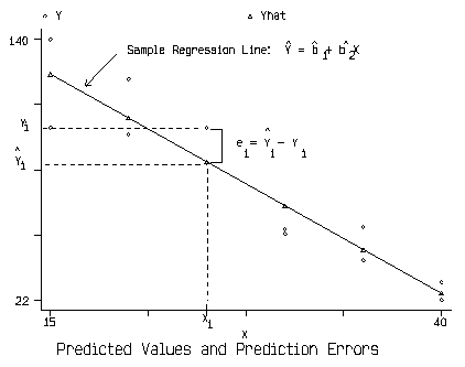
\(\hat{Y_i}\) is the value of Y we would expect from an observation with a value of \(X_i\).

\(e_i\) is the error for observation \(i\). How far off were we in our prediction?

The way we estimate \(\beta_0\) and \(\beta_1\) will determine how big our errors are on average.

There are a variety of ways we might find a line of best fit. A tempting one would be to minimize the sum of errors.

But positive errors cancel out negative errors, so there are many possible lines with an average error of 0.

OLS (Ordinary Least Squares) is the standard method for finding a line of best fit. It finds a line that will minimize the squared errors.
That is, it finds values of \(\beta_0\) and \(\beta_1\) that minimize the following equation:

\[\Sigma_i \varepsilon_{i}^2 = \Sigma_i (Y_i - \beta_0 - \beta_1 X_i)^2\]

Finding \(\beta_0\) and \(\beta_1\) results in estimates with a lot of nice properties that we will discuss in the future.