Spatial Analysis in R

Hannah Owens
05 March, 2024

The Plan

Agenda

Intro to GIS and Spatial Analysis
Case study: Sherman's Fox Squirrel

The Plan

Agenda

Intro to GIS and Spatial Analysis
Case study: Sherman's Fox Squirrel

Intended learning outcomes

Explain how R can be used for spatial analysis
Sketch out a workflow for analyzing and mapping spatial data in R

Intro to GIS and Spatial Analysis

What do you mean, GIS?

“a framework for gathering, managing, and analyzing spatial data”

GIS vs R

GIS	R
No programming knowledge needed	Repeatable and scaleable
Easy to create new spatial objects	Free and open-source

Spatial Data Types

Data types

Vector Data

Spreadsheets with a geometry column(s)
Vertices and paths

Vector Data: Points

X - Y coordinates in a spatial reference frame
- Generally latitude and longitude
- Careful! X = longitude, Y = latitude!
e.g. locality

Vector points

Vector Data: Lines

Links bewteen X - Y coordinates
Represent one-dimensional features
e.g. rivers, streets, movement paths

Vector points

Vector Data: Polygons

Connect X - Y coordinates and close the path
Represent two-dimensional features
e.g. conservation areas, country boundaries, distribution limits

Vector points

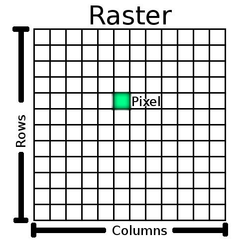
Raster Data

Made up of pixels
- Each pixel has a value
- Can be continuous or discrete
Many different file types
- GeoTIFF
- Ascii

Raster

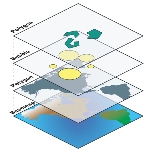
Comparing Vectors and Rasters

Vector	Raster
High geographical accuracy	Very good for representing remote sensing data
Efficient representation of hierarchical data	Performs well with map algebra
Used for measurements of proximity	Works well with continuous data

Mapping

Data visualization
Stack different data in layers

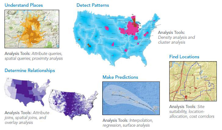
Simple Spatial Analysis

Overlay
- Intersection
- Data extraction
- Raster algebra
Proximity
- Distances (vectors)
- Interpolation (rasters)

Simple Spatial Analysis

Case Study

Sherman's Fox Squirrels

Some background

Subspecies of Fox Squirrel, Sciurus niger
Native to southeastern United States
Threatened by deforestation

The Plan

Load data
Manipulate data
Visualize data
Analyze data

5 Minute Break

If you haven't done so already:

Download data from Absalon
Install necessary packages

install.packages("terra")

Setting up and loading data

terra Package

Vector data
- Geometric operations (e.g. intersect and buffer)
Raster data
- Local, focal, global, zonal and geometric operations
Predict and interpolate using regression models
Processing of very large files is supported
- Using C++

terra

library(terra)
citation("terra")

To cite package 'terra' in publications use:

  Hijmans R (2024). _terra: Spatial Data Analysis_. R package version
  1.7-71, <https://CRAN.R-project.org/package=terra>.

A BibTeX entry for LaTeX users is

  @Manual{,
    title = {terra: Spatial Data Analysis},
    author = {Robert J. Hijmans},
    year = {2024},
    note = {R package version 1.7-71},
    url = {https://CRAN.R-project.org/package=terra},
  }

Basics of Loading Data: Vectors

Key function: vect()

vect()

 class       : SpatVector 
 geometry    : none 
 dimensions  : 0, 0  (geometries, attributes)
 extent      : 0, 0, 0, 0  (xmin, xmax, ymin, ymax)
 coord. ref. :

Basics of Loading Data: Vectors

From .csv file

#Read points and turn into shapefile
shermanSquirrels <- read.csv(file = "data/ShermanSquirrels.csv", header = T)

class(shermanSquirrels)

[1] "data.frame"

head(shermanSquirrels, 3)

        Species Longitude Latitude
1 Sciurus niger -83.36905 31.40090
2 Sciurus niger -82.60067 28.46997
3 Sciurus niger -81.46268 28.71139

Basics of Loading Data: Vectors

Converting a data.frame to a SpatVector

shermanSquirrelsShp <- vect(shermanSquirrels, geom = c("Longitude", "Latitude"))
shermanSquirrelsShp

 class       : SpatVector 
 geometry    : points 
 dimensions  : 35, 1  (geometries, attributes)
 extent      : -87.04154, -80.0361, 26.7061, 34.82  (xmin, xmax, ymin, ymax)
 coord. ref. :  
 names       :       Species
 type        :         <chr>
 values      : Sciurus niger
               Sciurus niger
               Sciurus niger

Basics of Loading Data: Vectors

Polygons from .shp files

# Reading shapefiles
florida <- vect("data/FloridaBound1/FLORIDA.shp")
florida

 class       : SpatVector 
 geometry    : polygons 
 dimensions  : 1, 4  (geometries, attributes)
 extent      : -1110383, 1298633, 77020.92, 2466420  (xmin, xmax, ymin, ymax)
 source      : FLORIDA.shp
 coord. ref. : NAD83(HARN) / Florida West (ftUS) 
 names       : OBJECTID  DATESTAMP SHAPE_AREA SHAPE_LEN
 type        :    <int>      <chr>      <num>     <num>
 values      :        1 2000/05/16   1.57e+12 2.834e+07

Basics of Loading Data: Rasters

Key function: rast()

rast()

class       : SpatRaster 
dimensions  : 180, 360, 1  (nrow, ncol, nlyr)
resolution  : 1, 1  (x, y)
extent      : -180, 180, -90, 90  (xmin, xmax, ymin, ymax)
coord. ref. : lon/lat WGS 84

Basics of Loading Data: Rasters

Raster from .tif files

# Read rasters
altitude <- rast("data/altitude.tif")

altitude

class       : SpatRaster 
dimensions  : 3000, 3000, 1  (nrow, ncol, nlyr)
resolution  : 0.01666667, 0.01666667  (x, y)
extent      : -100, -50, 0, 50  (xmin, xmax, ymin, ymax)
coord. ref. : lon/lat WGS 84 (EPSG:4326) 
source      : altitude.tif 
name        : ETOPO_2022_v1_60s_N90W180_bed 
min value   :                     -8461.562 
max value   :                      5424.277

names(altitude)

[1] "ETOPO_2022_v1_60s_N90W180_bed"

Challenge 1: Load spatial data

Now it's your turn! Load the point .csv, shapefile, and raster.

Bonus challenge: How many points are in the squirrel data?

Challenge 1: Load spatial data

# Points from .csv
shermanSquirrels <- read.csv(file = "data/ShermanSquirrels.csv",
                      header = T)
shermanSquirrelsShp <- vect(shermanSquirrels, 
                            geom = c("Longitude",
                                     "Latitude"))
paste0("There are ", 
       length(shermanSquirrelsShp), 
       " squirrels in the dataset.")

[1] "There are 35 squirrels in the dataset."