Whether designing an experiment to collect data or investigating trends in existing data, researchers will design a question to inform their efforts such as;
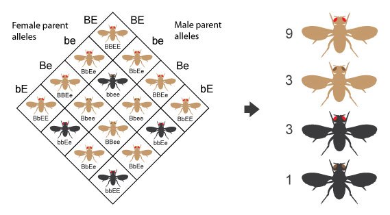
- “Is the rate of inheritance for two genes different from expected if they were unlinked?”
- “Is cancer incidence in mammals related to their litter size?”
Often, collecting data from the entirety of a population is infeasible. We are able to draw conclusions about the population by looking at a well-selected representative sample.
Hypothesis testing allows us to determine if a correlation in a sample is significant enough to draw a conclusion about the population, and to what degree that evidence is substantial.