Overview
Many “coding challenges” online will ask readers to create a Monte Carlo simulation to estimate the value of \(\pi\). The most popular method involves selecting a large number of points (x,y) from a square 2D grid, and then find the proportion of points that lie within a circle inscribed in the square. For a large population of points, the proportion of points inside the square that are also inside the circle should approach \(\frac{\pi}{4}\). Another popular approach is to simulate Buffon’s Needle, a famous 18th-century geometric problem. We will look at these and (many) other methods to estimate \(\pi\) in a Monte Carlo simulation in R.
Most of this was created in base R; the only libraries that I called were vioplot (for a “violin plot” interpretation of probability density plots) and DT (for formatting some graphics presented as tables.) In Python, you would need to call NumPy for some math functions (random number generation, trigonometry, combinatorics) and either matplotlib or seaborn for graphics (both of which support violin plots - in fact Seaborn is particularly good at making violin plots.)
Geometric interpretation: points in a square vs inscribed circle
In the graphic below, we picked 1000 points where the x- and y-coordinates can vary from 0 to 1 in a random uniform distribution. The circular arc defines points that lie within Pythagorean distance 1 of the origin; as we plot more and more points, the proportion of points (shaded red) that lie inside the arc should approach \(\frac{\pi}{4}\) (the ratio of the area of a 90\(^\circ\) arc of a unit circle to the area of a unit square.)

Out of 1000 trials, we got 767 successes, for a probability \(p\) = 0.767 which gives suggests that \(\pi \approx 4p\) = 3.068. The 95% confidence interval of the mean is 2.9631946 to 3.1728054.
It is easy to see why the “circle inside a square” method works and is popular, but is it the best way to estimate \(\pi\)? What might make one method be better than another?
Buffon’s Needle, with and without cheating
In the classic Buffon’s Needle problem, we have a needle (or some object of unit length and negligible width.) If we drop the needle onto lined paper, what is the probability that the needle will land such that it crosses a line? The problem can be generalized in such a way that the length of the needle and the spacing between the lines do not have to be the same; but for the case where they are equal, the probability that the needle lands on top a line is \(\frac{2}{\pi}\) so we will use that case to generate our Monte Carlo simulation.
A Monte Carlo approach based on Buffon’s Needle might go something like this:
- pick values from the range [0,0.5] to represent the distance from the center of the needle to the nearest line
- pick values from the range [0, 90\(^\circ\)] to represent the angle between the needle and the line
- use trig functions to locate the endpoints of the needle
- determine whether the endpoints of the needle are on opposite sides of the line
Sample code:
pi      <- atan(1)*4                 # have you no shame?!
centers <- runif(1E4, 0, +0.5)       # distance from center of needle to nearest line
angles  <- runif(1E4, 0, pi/2)       # angle can be in range 0-90 degrees, but that's pi/2 radians
left    <- centers + sin(angles)/2   # find endpoints of the needle
right   <- centers - sin(angles)/2

crosses <- floor(left)!=floor(right) # are the endpoints on opposite sides of the line
prob <- mean(crosses)                # probability of cross = 2/pi
pi_est <- 2/prob
pi_est
[1] 3.121099So … in a problem where we are trying to run a simulation to estimate \(\pi\), we started by feeding it the numerical value for \(\pi\) so that we could define the range of allowable angles. If you defined the range as 0-180 (degrees) instead, you’d still have to convert them to radians (i.e. divide by \(\frac{180}{\pi}\)) before feeding them into the sine function. Can we make a Buffon’s Needle simulation that avoids this self-referential problem?
Fortunately there IS a circle picking method that allows you to select points on a circle from a random uniform distribution, but using Cartesian coordinates as inputs instead of angles. Without getting too far into the weeds about why this works, here is the method, first formulated by the great Hungarian-American mathematician and physicist John von Neumann:
choose paired values \(x_1\) and \(x_2\) independently from uniform distribution [-1,+1]
REJECT any pairs where \(x_1^2 + x_2^2 \geq 1\)
for the remaining pairs, map to points on the unit circle using these functions:
x = \(\frac{x_1^2 - x_2^2}{x_1^2+x_2^2}\)
y = \(\frac{2x_1 x_2}{x_1^2+x_2^2}\)
Here is a plot of 1000 points based on this method. The pink points were mapped from pairs that followed the rule \(x_1^2 + x_2^2 < 1\), and they conform to a uniform distribution of points on the circle. The black points are the rejects, the ones where \(x_1^2 + x_2^2 \geq 1\); while they do all lie on the circle, they are concentrated near the north and south poles, so to speak, rather than being equally likely to land anywhere on the circle. So the idea is to keep the pink points and reject the black ones.

We can rewrite our Buffon’s Needle code using the pink points as the basis for the angle orientation of the needle. Now we can estimate \(\pi\) without referring to \(\pi\) at any point:
# Buffon's needle without cheating
centers <- runif(1E4, 0, +0.5)
x1 <- runif(1E4, -1, +1)
x2 <- runif(1E4, -1, +1)
test <- (x1^2 + x2^2 >= 1)
x_circ <- (x1^2 - x2^2)/(x1^2+x2^2)
y_circ <- 2*x1*x2 / (x1^2+x2^2)

left <- centers + y_circ/2
right <- centers - y_circ/2
crosses <- floor(left)!=floor(right)
crosses <- crosses[test==FALSE]
prob <- mean(crosses)
pi_est <- 2/prob
pi_est
[1] 3.174201So it works … but note that the process of rejecting the points such that \(x_1^2 + x_2^2 \geq 1\) is identical to the “circle area” method that we already covered; you will end up keeping \(\frac{\pi}{4}\) of the pairs, and reject \(1-\frac{\pi}{4}\) of the pairs. You could have just used that as your \(\pi\) estimate and skipped the whole Buffon’s Needle simulation!
Conclusion: Buffon’s Needle is an unsatisfying way to simulate \(\pi\) in R or Python. You have to either use \(\pi\) itself in your code, or else resort to a workaround that by itself is sufficient to simulate \(\pi\) without even doing the needle part. Let’s look at some other methods.
Monte Carlo simulation as the “poor man’s integration”
Reviewing the graphic above, the heavy black arc that defines the boundary between success and failure can be described by the function \(y = \sqrt{1-x^2}\). We can calculate \(\pi\) by finding the area under the curve from 0 to 1, i.e.
\(A = \int_{0}^{1} \sqrt{1-x^2} dx = \frac{\pi}{4}\)
Even if you don’t know how to perform integral calculus, or if you just don’t know how to evaluate this particular integral, you still have the opportunity to use a Monte Carlo simulation as an alternative way to estimate the area under a curve. We can estimate the area under the curve \(y = \sqrt{1-x^2}\) between 0 and 1 by choosing a series of values from a random uniform distribution in [0,1], then evaluating \(\sqrt{1-x^2}\) for each of those values, then finding the mean of all those evaluations, and then finally multiplying the mean by the width of the range (in this case 1-0 = 1.) We already know that the area should be \(\frac{\pi}{4}\) since it represents a quadrant of a unit circle, so we can use this method to estimate \(\pi\).
Let’s try that for approach for a series of 1000 observations, and this time, let’s also calculate the running mean and the running 95% confidence interval bounds as we take more and more samples; we should see the mean (black) approach the heavy line (which represents the true value of \(\pi\) = 3.1415927…) and the CI bounds (red and green) start to constrict around the mean. I will include the code to generate the first graphic below.
# "a" is a vector of 1000 random values 0-1 already defined in the setup chunk
# z95 (approx 1.96) is the critical z for two-tailed 95% conf int

circ <- 4*sqrt(1-a^2)                       # estimates for pi
n <- seq_along(circ)                        # index for running totals
CM <- cumsum(circ)/n                        # running mean of estimates
CS <- cumsum(circ**2)/n                     # running mean of squared estimates
CV <- CS - CM^2                             # V(x) = E(x^2) - [E(x)]^2
Csd <- sqrt(CV)                             # sd(x) = sqrt(V(x))
Clow <- CM - z95 * Csd/sqrt(n)              # running 95% confidence intervals
Cupp <- CM + z95 * Csd/sqrt(n)

# add mean and 95% CI bounds to a dataframe for presentation later
df[nrow(df) + 1,] = c("circle area", CM[1000], Clow[1000], Cupp[1000])

# now add the plot
plotDF <- data.frame(CM, Clow, Cupp)
matplot(plotDF, pch = 19, type = "b", cex=0.5,
        xlab = "trials", ylab = "value",
        ylim = c(2.5, 3.5),
        main = "Monte Carlo simulation based on area under the curve")
abline(h=pi, lwd =2, col = "darkgreen")
This method converges to \(\pi\) a little faster than the 2D points method; we estimated \(\pi\) = 3.1061195 with a 95% CI of 3.0496448 to 3.1625943.
Inverse Trig Functions
Note that the formula for arcsine (inverse sine, i.e. given some value -1 to +1, what angle has that value as a sine) can be written
sin\(^{-1}\)(z) = \(\int_{0}^{z} \frac{dx}{\sqrt{1-x^2}}\)
sin\(^{-1}\)(1) = \(\frac{\pi}{2}\) is the same thing as saying that a 90\(^{\circ}\) angle (which is \(\frac{\pi}{2}\) radians) has a sine of 1, so we can write
sin\(^{-1}\)(1) = \(\int_{0}^{1} \frac{dx}{\sqrt{1-x^2}} = \frac{\pi}{2}\)
What happens if we use this integral to estimate \(\pi\)? So our approach will be: pick 1000 values in a uniform distribution [0,1], find \(\frac{2}{\sqrt{1-x^2}}\) for each value and find the mean.

We got an estimate of \(\pi\) = 3.143965 with a 95% CI of 2.9664261 to 3.3215038. The problem here is that the denominator can get arbitrarily close to 0, producing some extremely large values that are creating occasional spikes in our rolling averages.
We can improve on this by considering that sin\(^{-1}\)(1/2) = \(\int_{0}^{1/2} \frac{dx}{\sqrt{1-x^2}} = \frac{\pi}{6}\) that is, the sine of 30\(^{\circ}\) = \(\frac{1}{2}\). Now the largest allowable value for our random numbers is \(\frac{1}{2}\) which makes it impossible to have a denominator very close to zero. (Note: Niven’s Theorem says that sin(0) = 0, sin(30) = 0.5 and sin(90) = 1 are the only cases where you have both a rational angle in degrees and a rational sine.)

That’s a big improvement: now we estimated \(\pi\) = 3.1470347 with a 95% CI of 3.1385526 to 3.1555168.
The arctangent formula also avoids the problem we encountered with the arcsin(1) integral, in that its denominator can never be less than 1. The integral looks like this:
tan\(^{-1}\)(z) = \(\int_{0}^{z} \frac{dx}{1+x^2}\)
tan\(^{-1}\)(1) = \(\frac{\pi}{4}\) is the same thing as saying that a 45\(^{^\circ}\) angle has a tangent of 1, so we can write
tan\(^{-1}\)(1) = \(\int_{0}^{1} \frac{dx}{1+x^2} = \frac{\pi}{4}\)
Let’s try it:

For the arctangent integral, we estimated \(\pi\) = 3.1202969 with a 95% CI of 3.0796077 to 3.1609861.
How about combining two arctangents? Machin’s formula
tan\(^{-1}(\frac{1}{5})\) - tan\(^{-1}(\frac{1}{239}) = \frac{\pi}{4}\)
was used to calculate \(\pi\) to 527 decimal places in the 19th century.

Now we’re really getting somewhere: with the same 1000 trials, we estimated \(\pi\) = 3.140202 with a 95% CI of 3.1379133 to 3.1424908.
Other Integrals
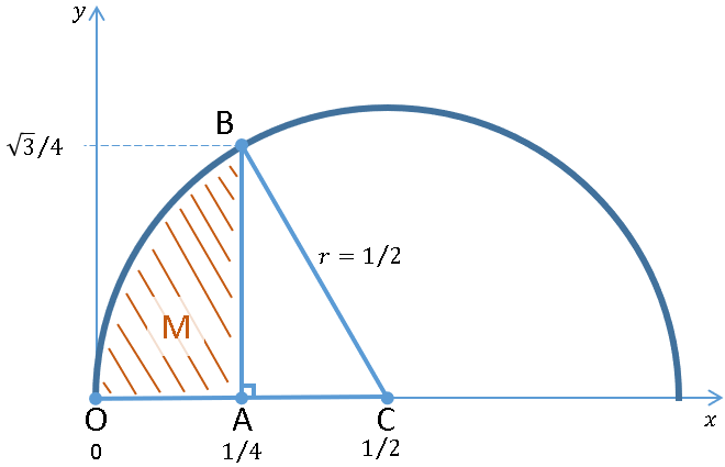
In 1665, Isaac Newton calculated \(\pi\) using the method shown below: the circle with a radius of \(\frac{1}{2}\) has area \(\frac{\pi}{4}\). The angle OCB is 60 degrees, so it subtends \(\frac{1}{6}\) of the circle (area \(\frac{\pi}{24}\).) We can get the area of the triangle ABC = \(\frac{\sqrt{3}}{32}\) by Pythagorean theorem, so \(\frac{\pi}{24}\) = \(\frac{\sqrt{3}}{32}\) + the curved area M, whose area = \(\int_{0}^{1/4} \sqrt{x-x^2}dx\)


With this integral, we estimated \(\pi\) = 3.1478126 with a 95% CI of 3.1098916 to 3.1857337.
One last example: the 1968 Putnam Competition exam included a problem asking how to use the integral below to prove that \(\pi < \frac{22}{7}\):
\(\int_{0}^{1} \frac{x^4(1-x)^4}{1+x^2} dx\)
The answer lies in the fact that the integral evaluates to \(\frac{22}{7} - \pi\). (The proof of this result has its own page on Wikipedia.) Using this formula as the basis for a Monte Carlo simulation is almost cheating, because we already know that the result is going to be very close to \(\pi\), but let’s try it.

With the same 1000 trials, we estimated \(\pi\) = 3.1416542 with a 95% CI of 3.1415821 to 3.1417263.
Summary of integral methods
For each of the seven integral methods described above, we generated 1000 different estimates for \(\pi\) and then found the means of those estimates. Let’s look at the range of estimates that each method produces. The sin\(^{-1}\)(1)=\(\frac{\pi}{2}\) method can’t produce an estimate below 2, but there is no upper bound on how high of an estimate it can produce. By contrast, the sin\(^{-1}\)(1/2)=\(\frac{\pi}{6}\) method can only produce estimates for \(\pi\) ranging from a low of 3 to a high of 2\(\sqrt{3}\) = 3.46+, so we achieve faster convergence. The Machin and Putnam integrals can only produce estimates so close to \(\pi\) that the heavy red line that we plotted to represent \(\pi\) itself obscures most or all of their range.

Ramanujan’s amazing equation
Finally, for something completely different: the Indian prodigy Srinivasa Ramanujan (1887-1920) discovered some remarkable infinite series for \(\pi\), including this astounding result:
\(\frac{1}{\pi} = \sum_{n=0}^{\infty} \binom{2n}{n}^3 (\frac{6n+1}{2^{8n+2}})\)
Flajolet et al. 2010 showed how this formula can be converted into a dice-rolling, coin-flipping Monte Carlo simulation for \(\pi\).
take a d4 (tetrahedral) die and roll it repeatedly. Keep track of the number of times you roll a “1”; continue rolling until you have failed twice. (For example, if you rolled the sequence 1-1-2-1-4 you would note that you rolled three “1”s before failing twice.)
take a pair of regular d6 dice and roll them just once. If you roll a sum of 5, 6, 7 or 8 (an event that will occur with probability 5/9) increase your score from step 1 by a single point. Let’s call your score at this point \(t\).
Get \(2t\) fair coins and flip them all. If you get exactly \(t\) heads and \(t\) tails, flip them all again. If you succeed in getting \(t\) heads and \(t\) tails a second time, flip them all a third time. If that third flip also produces \(t\) heads and \(t\) tails, then the entire trial is to be treated as a success.
This process is analogous to the Ramanujan sum and thus will, incredibly, produce successful trials with a probability of exactly \(\frac{1}{\pi}\). How can a process that involves flipping coins and rolling dice have a probability that works out to a transcendental number? Any event that involved a strictly finite number of dice rolls and/or coin flips would necessarily have a rational probability; but remember that you get to keep re-rolling the d4 indefinitely as long as you keep rolling “1”, so the d4 die part of the process creates a geometric series with an infinite number of terms. As for the coin flips, the probability that \(2t\) fair coins will produce \(t\) heads is \(\binom{2t}{t} / 2^{2t}\) so you can see where that part of the formula comes from, at least.
z=0                    # running total of successes
n = 1E5                # number of trials

for (x in 1:n){

# roll the dice
d1 <- floor(log(runif(1,0,1))/log(0.25))  # 1s before first failure
d2 <- floor(log(runif(1,0,1))/log(0.25))  # 1s before second failure
d3 <- sum(runif(1,0,1)>= 4/9)             # extra point 5/9 chance of success
t  <- d1+d2+d3                            # we are going to flip 2t coins

# flip the coins
f1 <- (sum(runif(2*t, 0,1) >=0.5) == t)   # simulate the coin flips once ...
f2 <- (sum(runif(2*t, 0,1) >=0.5) == t)   # twice ...
f3 <- (sum(runif(2*t, 0,1) >=0.5) == t)   # and thrice
if(sum(f1,f2,f3) == 3) {z=z+1}
}

pi <- n/z                    # simulated value of pi
In the example above, our simulation succeeded at a probability of 0.32109 and our estimate for \(\pi\) is the reciprocal of that, 3.1143916.
To try to get a handle on what’s going on here, the table below shows the theoretical probability (P\(_t\)) for each value of \(t\) after the dice rolling part of the algorithm, and the probability (P\(_s\)) of the coin flip exercise succeeding (i.e. get \(t\) heads and \(t\) tails from 2\(t\) coins, three times in a row) given \(t\). (Note that for \(t\)=0 you automatically succeed at getting 0 heads from 0 flips.) The table can go on forever, of course, but even summing the terms up to \(t\)=6, column P adds up to 0.318302+. The reciprocal of that value, 3.14167 … is already close to \(\pi\) and will get closer as you add more terms to the series.
func <- function(x){(9/16)*(x+1)*4^(-x)}   # prob of rolling "1" x times before failing twice
t <- seq(0,6)
P_t <- mapply(func,t)*4/9 + mapply(func,t-1)*5/9
P_s <- (choose(2*t,t)/2^(2*t))^3
P   <- P_t * P_s
data.frame(t, P_t, P_s, P) %>%
        datatable(options = list(dom = 't'), rownames = FALSE) %>%
        formatRound(columns=c(2,3,4), digits=6)
Recommendations
Of all the methods surveyed, I think my favorite is the one based on
sin\(^{-1}\)(1/2) = \(\int_{0}^{1/2} \frac{dx}{\sqrt{1-x^2}} = \frac{\pi}{6}\);
it’s a good combination of easy to code, fast to run and fast to converge. Let’s see what happens if we let this method stretch its legs a little and run for a million trials.
From one million trials, we estimated \(\pi\) = 3.1414017 with a 95% CI of 3.1411397 to 3.1416637.