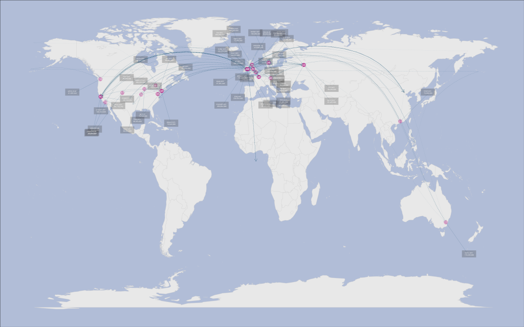
A Traceroute Map of the Top 50 websites in R
I came up this project to improve the things I'm bad at in R; namely interfacing with online API's, extracting objects from messy data and iteratively creating ggplot2 images. Again, I'm happy with the result, even if the image is blatantly bing-esque. The plot was created by tracerouting the current top fifty websites, geolocating the IP address obtained and plotting the result.
Click here to view the full-size image with visible labels.
Traceroute is a diagnostic tool which displays the path across an IP network. It works by sending echo request packets to a host, determining the intermediate routers by adjusting the hop limit incrementally. The final host will return the echo reply message. The IP addresses can be then geolocated with one of several geolocation API's. These aren't 100% accurate, but they can often pinpoint the city an IP seems to be located in based on database lookup.
When I began working on this project I was worried that I would get a lot of the hosts placed in the middle of the ocean. Fortunately, there are only a few intermediate servers placed in odd locations.
The map shows that most host echo replies were sent from West Europe (including Ireland, my home country) and the USA, with some hosts further afield in China and Australia. Not surprisingly there is a large cluster of hosts located in California. The intermediate routers are mostly occluded as they tend to be located close the the destination host. Keep reading if you are interested in the code behind the map.
First, some housekeeping. I used a few external libraries to map the traceroute data. I chose to use geosphere instead of implementing my own Great Earth Circle function to simplify my code. I also bound some common functions to an alternate name; writing length(x) always felt unnatural to me.
require(ggplot2)
require(stringr)
require(RCurl)
require(geosphere)
require(Cairo)
l <- base::length
n <- base::nrow
m <- base::ncol
mod <- base::"%%"
The raw data (a list of the top 50 websites and the number unique visitor to each) came from google's ad planner page, which I downloaded from the site, tidied up and imported into R as a data frame. I retyped the data as R object code below.
websites <- c("facebook.com", "youtube.com", "yahoo.com", "live.com",
    "msn.com", "wikipedia.org", "blogspot.com", "baidu.com", "microsoft.com",
    "qq.com", "bing.com", "ask.com", "adobe.com", "taobao.com", "twitter.com",
    "youku.com", "soso.com", "wordpress.com", "sohu.com", "hao123.com", "windows.com",
    "163.com", "tudou.com", "amazon.com", "apple.com", "ebay.com", "4399.com",
    "yahoo.co.jp", "linkedin.com", "go.com", "tmall.com", "paypal.com", "sogou.com",
    "ifeng.com", "aol.com", "xunlei.com", "craigslist.org", "orkut.com", "56.com",
    "orkut.com.br", "about.com", "skype.com", "7k7k.com", "dailymotion.com",
    "flickr.com", "pps.tv", "qiyi.com", "bbc.co.uk", "4shared.com", "mozilla.com",
    "ku6.com", "imdb.com", "cnet.com", "babylon.com", "mywebsearch.com", "alibaba.com",
    "mail.ru", "uol.com.br", "badoo.com", "cnn.com", "myspace.com", "netflix.com",
    "weather.com", "soku.com", "weibo.com", "renren.com", "rakuten.co.jp", "17kuxun.com",
    "yandex.ru", "booking.com", "ehow.com", "bankofamerica.com", "58.com", "zedo.com",
    "345.com")

uniqueVisitors <- c(8.5e+08, 8e+08, 5.9e+08, 4.9e+08, 4.4e+08, 4.1e+08,
    3.4e+08, 3e+08, 2.5e+08, 2.5e+08, 2.3e+08, 1.9e+08, 1.6e+08, 1.6e+08, 1.6e+08,
    1.4e+08, 1.4e+08, 1.3e+08, 1.2e+08, 1.2e+08, 1.1e+08, 1.1e+08, 1.1e+08,
    1.1e+08, 9.8e+07, 8.8e+07, 8.2e+07, 8.1e+07, 8e+07, 7.4e+07, 7.3e+07, 7.3e+07,
    7.2e+07, 6.7e+07, 6.6e+07, 6.6e+07, 6.6e+07, 6.6e+07, 6.6e+07, 6.2e+07,
    6.1e+07, 6.1e+07, 6.1e+07, 6.1e+07, 6e+07, 6e+07, 5.9e+07, 5.6e+07, 5.6e+07,
    5.5e+07, 5.1e+07, 5e+07, 5e+07, 5e+07, 5e+07, 5e+07, 4.9e+07, 4.9e+07, 4.6e+07,
    4.6e+07, 4.6e+07, 4.6e+07, 4.5e+07, 4.5e+07, 4.2e+07, 4.2e+07, 4.2e+07,
    4.2e+07, 4.1e+07, 4.1e+07, 4.1e+07, 4.1e+07, 4.1e+07, 4.1e+07, 4.1e+07)
Acquiring the IP addresses was pretty easy; I simply ran the shell command tracert -d URL over a vector of URLs above. It took a long time to complete, but the -d parameter helped speed things up by preventing the intermediate routers being resolving to their names.
I used a regular expression to match and pull the ip addresses from the text printed to the shell. The str_match function in stringr helped, as sometimes the native string functions act “surprisingly” to say the least.
ServerIP <- function(websites) {

    pathList <- list()
    websites <- paste(" ", websites)

    patternIP <- "([0-9]+\\.){3}[0-9]+"

    for (site in 1:l(websites)) {

        pos <- 1
        processedIP <- ip <- list()
        websiteURL <- websites[site]

        cat(site, "/", l(websites), " tracing", websiteURL, " IP address(es) \n",
            sep = "")

        # 2. use tracert to find the IP addresses

        addressIP <- system(command = paste("tracert -d", websiteURL, sep = ""),
            intern = TRUE)

        pathIP <- rep(0, l(addressIP))

        for (i in 1:l(addressIP)) {

            # 3. use pattern matching to extract the IP addressed from the tracert
            # data

            line <- addressIP[i]

            matchIP <- str_match(pattern = patternIP, string = line)[, 1]

            if (!is.na(matchIP)) {

                pathIP[pos] <- matchIP
                pos <- pos + 1

            }

        }

        # 4. add each path of IP's to a list

        pathList[[site]] <- pathIP[1:(pos - 1)]

    }

    return(pathList)

}
Now it's time to pass the IP addresses from the traceroute to the online geolocation API. As with my last project, I'm using a basic stream capturing function combined with RCurl to get the data, before reimporting it to extract the coordinates.
GeoAPIWrite <- function(x) {

    if (nchar(x) > 0) {

        write.table(file = "PathGeodata.txt", x, row.names = FALSE, col.names = FALSE,
            append = TRUE)
    }
}
This function converts each IP to a query for hostip.info, which will return the longitude/latitude coordinates if they are available.
GeoAPIQueries <- function(addresses) {

    return(lapply(X = addresses, FUN = function(x) {

        paste("http://api.hostip.info/get_html.php?ip=", x, "&position=true",
            sep = "")
    }))

}
The queries are returned in JSON format, a friendly XML alternative. This made it easy to extract the coordinates; it was simply a matter of looking for the Longitude: and Latitude: keys.
ServerLocations <- function(queries) {

    download.file(url = "http://curl.haxx.se/ca/cacert.pem", destfile = "cacert.pem")

    siteCoordinates <- list()

    for (site in 1:l(queries)) {

        pos <- 1
        pathLongitude <- pathLatitude <- rep(0, 150)

        # 1. extract each set of path queries

        pathQueries <- queries[[site]]

        cat(site, "/", l(queries), " downloading geolocation data\n", sep = "")

        for (i in 1:l(pathQueries)) {

            query <- pathQueries[i]

            # 2. get data from the geolocation service

            locationIP <- getURL(url = query, cainfo = "cacert.pem")

            locationIP <- gsub("\n", " ", locationIP, fixed = TRUE)
            locationIP <- unlist(strsplit(locationIP, " "))

            latitude <- locationIP[which(locationIP == "Latitude:") + 1]

            longitude <- locationIP[which(locationIP == "Longitude:") + 1]

            # 3. if longitude is not empty, neither is latitude

            if (longitude != "") {

                pathLongitude[pos] <- longitude
                pathLatitude[pos] <- latitude
                pos <- pos + 1

            }

        }

        pathCoordinates <- rbind(pathLongitude[1:(pos - 1)], pathLatitude[1:(pos -
            1)])

        siteCoordinates[[site]] <- pathCoordinates

    }

    return(siteCoordinates)

}
Now for the tricky part; making a custom graphic. The ggplot function is very customisable, and capable of easily creating great graphics. The price you pay for this flexibility is verbosity (if you override many default settings). I ended up with 200 lines of code for the main graphic, although it's probably shortened in the final markdown document due to the loss of my esoteric code indentation.
To minimize occlusion, I made the great circle lines connecting each intermediate router transparent, with earlier steps in the path much less prominent. I also added arrows to clarify the packet flow direction. It took me a long time to figure out the best way to show the site name and popularity; in the end I settled on using a label. The only downside was that it didn't entirely fix the occlusion problem, and I didn't want to write a vertice layout function as in igraph. My fix was to randomly generate the positions, make 20 plots and pick the best. It worked, although it was a mechanical turk solution.
LocationsPlot <- function(siteCoordinates, usage, myCoordinates = c(-7.2,
    53.35)) {

    cat("creating map...\n")

    # 1. plot the world map

    world <- map_data("world")
    LineStore <- c(0, 0)
    LineLength <- rep(0, l(siteCoordinates))

    # 2. turn of the background panels and axes, and tweak some of the colours

    newPlot <- ggplot(legend = FALSE) + geom_polygon(data = world, aes(x = long,
        y = lat, group = group), fill = "#E8E8E8", colour = "#D3D3D3") + opts(plot.background = theme_rect(fill = "#B1BDD7"),
        panel.background = theme_blank(), panel.border = theme_blank(), panel.grid.major = theme_blank(),
        panel.grid.minor = theme_blank(), axis.line = theme_blank(), axis.ticks = theme_blank(),
        axis.text.x = theme_blank(), axis.text.y = theme_blank(), axis.title.x = theme_blank(),
        axis.title.y = theme_blank())

    # 2. iteratively plot each path

    for (path in 1:l(siteCoordinates)) {

        cat(path, "/", l(siteCoordinates), "plotting website traceroute (memory usage =",
            memory.size(), "Mb)\n")

        pathCoordinates <- unname(cbind(myCoordinates, siteCoordinates[[path]]))

        pathCoordinates <- apply(pathCoordinates, c(1, 2), as.numeric)

        for (i in 1:(m(pathCoordinates) - 1)) {

            point1 <- pathCoordinates[, i]
            point2 <- pathCoordinates[, (i + 1)]

            # 3. for each point pair in path, constuct a great earth circle

            geoConnection <- gcIntermediate(p1 = as.vector(unlist(point1)),
                p2 = as.vector(unlist(point2)), n = 13, addStartEnd = TRUE)

            lineDataframe <- data.frame(x = geoConnection[, 1], y = geoConnection[,
                2], stepLine = rep(i, n(geoConnection)))

            step <- m(pathCoordinates) - i + 1

            # 4. plot the great circle using geom_path, with arrows and alpha shading

            newPlot <- newPlot + geom_path(show_guide = FALSE, data = lineDataframe,
                aes(x, y, alpha = 1/(3 * max(stepLine) + 3)), colour = "#004366",
                size = 0.15, linetype = "longdash", arrow = grid::arrow())

            if (i != (m(pathCoordinates) - 1) && i != 1) {

                # 5. add a point for each intermediate router

                newPlot <- newPlot + geom_point(show_guide = FALSE, data = data.frame(x = point1[1],
                  y = point1[2], noSteps = step), aes(x, y, alpha = I(1/noSteps^2)),
                  colour = "grey", size = 3)
            } else {

                # 6. add a bigger point for the destination host

                if (i == (m(pathCoordinates) - 1)) {

                  x2 <- point1[1] + (22 * cos(sample(1:360, size = 1)))
                  y2 <- point1[2] + (22 * cos(sample(1:360, size = 1)))

                  newPlot <- newPlot + geom_point(show_guide = FALSE, data = data.frame(x = point1[1],
                    y = point1[2]), aes(x, y), colour = "#B62084", size = 11,
                    alpha = I(1/2)) + annotate("text", label = path, x = point1[1],
                    y = point1[2], colour = "white", size = 6) + geom_line(data = data.frame(x = c(point1[1],
                    x2), y = c(point1[2], y2)), aes(x, y), colour = "#004366",
                    alpha = I(1/4)) + geom_rect(data = data.frame(xmin = x2 -
                    5.5, xmax = x2 + 5.5, ymin = y2 - 1, ymax = y2 + 3), aes(xmin = xmin,
                    xmax = xmax, ymin = ymin, ymax = ymax), alpha = I(1/4)) +
                    annotate("text", x = x2, y = y2 + 1, label = paste(websites[path],
                      "\n", format(usage[path], big.mark = ",", scientific = FALSE)),
                      size = 3.3, colour = "white")

                }

            }

        }

    }

    print(newPlot)

}
Finally, I draw the graphc using the cairo device. This graphic device supports antialaising, unlike the default graphic.
data <- ServerIP(websites)
data <- GeoAPIQueries(data)
data <- ServerLocations(data)

CairoPNG("testPlot5.png", width = 2 * 1680, height = 2 * 1050)

    LocationsPlot(data[1:50], uniqueVisitors[1:50])

graphics.off()
If I was to redo the project, I would focus more on adding data non-iteratively to ggplot2; on my 32-bit OS I ran into memory limits for large data sets. Still, overall it was fun way to spend a few hours. Feel free to use the code(preferably with permission). Thanks to the authors of the pages I used, and hostip.info for their api.