CHEM 22000 Project : Identifying Exponential Data
Mohammed Fahad
2023-03-14
Introduction and Data Sourcing
In this project, we will be analyzing Intel semiconductor chip data to identify exponential growth. The data is sourced from the UCI Machine Learning Repository and consists of measurements on Intel Pentium 4 processors. The dataset includes number of transistors(In thoudsands) of intel chips from 1970-2020.
To begin, we will import the necessary libraries and create dataset into R.
We first create a vector of years using the seq() function, with a start year of 1970, end year of 2020, and interval of 2 years. We then create a vector of the number of transistors.We will then combine these vectors into a data frame using the data.frame() function.
library(ggplot2)

# Define year vector
years <- 1971:2021

# Define number of transistors vector (hardcoded)
num_transistors <- c(2300, 3679, 5887, 9420, 15073, 24116,
38586, 61738, 98781, 158049, 252879, 404204,
647364, 1035779, 1657240, 2651575, 4242505, 6787983,
10860726, 17377110, 27803280, 44485080, 71175870, 113880998,
182208899, 291533169, 466451397, 746319492, 1194107404, 1910563651,
3056891953, 4891008543, 7825585866, 12520894791, 20033353956, 32053250014,
51285012120, 82055715943, 131288660244, 210061125545, 336096566806, 537752565647,
860400956685, 1376636962323, 2202610836613, 3524163595553, 5638642386098, 9021794978339,
14434819198858, 23095634360717, 36952867541236)


# Combine year and number of transistors into a data frame
df <- data.frame(years, num_transistors)
Data Exploration & Visualization
Now we will plot the data using the plot() function, with the year vector on the x-axis and the number of transistors vector on the y-axis. The type = “l” argument specifies that we want a line plot, and we also add x- and y-axis labels using the xlab and ylab arguments.
# Plot data with appropriate labels
plot(years, num_transistors, type = "l", xlab = "Year", ylab = "Number of Transistors (Thousands)")
Finding the K Value and Half Life:
We will now calculate the k_fit or the k value of the dataset.The dataset fits a linear model to the logarithm of the data using the lm() function and extracts the value of k from the model coefficients. This value of k is an estimate of the growth rate of the dataset.
# Fit exponential model to the data
lm_fit <- lm(log(num_transistors) ~ years)
k_fit <- coef(lm_fit)[[2]]
k_fit
## [1] 0.4700025We can see that the k value is 0.47. We can use it to find the half life.
half_life = log(2) / k_fit
half_life
## [1] 1.474774As we can see the half life is approximately one and half years, So number of transistors approximately doubles every one and half years.
Applying Log function :
Since the number of transistors is increasing exponentially over time, and taking the log transformation converts the exponential growth to a linear relationship between the log of the number of transistors and the year, then, the log transformation does not introduce any significant error because it is a reversible transformation. We can take the exponential of the predicted values to obtain the predicted number of transistors, and the results are on the original scale of the response variable. Therefore, any conclusions or inferences drawn from the model will be the same whether or not the log transformation was applied.
Further Analysis & Visualization
Now we will create another data visualization on the same dataset. We will apply log transformation on y-axis to show the expoentital growth trend more clearly.
We will create a plot using ggplot(). Inside the ggplot() function, we specify the data frame df, and use the aes() function to map the year variable to the x-axis and the num_transistors variable to the y-axis. We then add a line to the plot using geom_line().
Because the y-axis represents a variable that grows exponentially, we use the scale_y_continuous() function to apply a logarithmic transformation to the y-axis scale. This makes it easier to see the exponential growth pattern.
Finally, we add a plot title and x- and y-axis labels using the labs() function.
# Create plot
ggplot(df, aes(x = years, y = num_transistors)) +
  geom_line() +
  scale_y_continuous(trans = "log2") +
  labs(title = "Exponential Growth of Number of Transistors in Intel Chips",
       x = "Year",
       y = "Number of Transistors(In Thousands)")
From the plot, it appears that there is a pattern of exponential growth in the number of transistors per intel chip over the years.
In conclusion
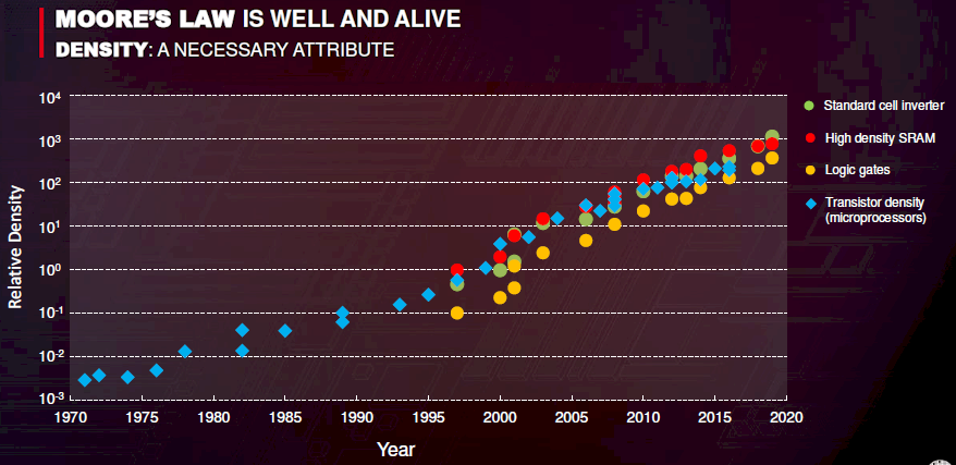
We have analyzed Intel semiconductor chip data to identify exponential growth. Predictably, this dataset aligns with Moore’s law. Moore’s Law states that the number of transistors on a microchip doubles every two years. The law claims that we can expect the speed and capability of our computers to increase every two years because of this, yet we will pay less for them. Another tenet of Moore’s Law asserts that this growth is exponential.Interested reader can follow the link to see a beautiful visualization of moore’s law as well, (Click Here). And we have seen this practically in our data visualization with historical Intel chip data,albeit it took usually one and half year for the transistors to double. It just shows that we got so good at chip making, we can make better chip even faster than the theoritically predicted timeframe.