ANLY 512 Problem Set 2
Introduction to Data Visualization
Carlos Borgonovo
2023-02-14
Directions
In this chapter we discussed why well-designed data graphics are important and we described a taxonomy for understanding their composition.
The objective of this assignment is for you to understand what characteristics you can use to develop a great data graphic.
Each question is worth 5 points.
To submit this homework you will create the document in Rstudio, using the knitr package (button included in Rstudio) and then submit the document to your Rpubs account. Once uploaded you will submit the link to that document on Canvas. Please make sure that this link is hyper linked and that I can see the visualization and the code required to create it.
Question #1
Answer the following questions for this graphic Relationship between ages and psychosocial maturity
knitr::include_graphics("http://ars.els-cdn.com/content/image/1-s2.0-S1043276005002602-gr2.jpg")
- Identify the visual cues, coordinate system, and scale(s)
Visual Cues: The graph above includes a few visual cues including color (we can see the bars are green and pink), numerical visual cues such as length and position.
Coordinate System: as seen in the graph, the relationship between age and physiological maturity is a Cartesian coordinate system (x,y)
Scales: The graph has two different scales - on the x-axis the graph has a time scale (which is also numeric) in which time is identified on a backward basis starting 20,000 years ago and ending right now. On the other hand the graph scale on the y-axis is linear numeric (age) starting at age zero and ending at age 20.
- How many variables are depicted in the graph? Explicitly link each variable to a visual cue that you listed above.
There are a total of 4 different variables that are depicted in the graph above (for “mismatch” and “physiological maturation”). The variables are 1) age on the y-axis, 2) time on the x-axis 3) physiological maturation depicted by the pink bars and 4) menarche depicted by the green bars.
- Critique this data graphic using the taxonomy described in the lecture.
The graph allows us to see the evolution and trend of both menarche and physiological maturation through time using different bars and colors, which allows us to change how both have evolved differently through time. Something we can notice from the graph is how menarche and physiological maturation through history have mostly happened at a similar time, but this has dispersed significantly over the last 200 years, with physiological maturation happening at a significantly older age than menarche.
Question #2
Answer the following questions for this graphic World’s top 10 best selling cigarette brands 2004-2007
- Identify the visual cues, coordinate system, and scale(s)
Visual Cues: Some fo the visual cues that are present of the “World’s Top 10 Best Selling Cigarette Brand” include color (the different cigarette brands are all depicted in different colors) and length (each cigarette brand has visibly a different length).
Coordinate System: as seen in the graph, the coordinate system is a cartesian coordinate system (x,y).
Scales: the graph has a categorical scale on the y-axis with the different cigarette brand names on that axis, and numerical scale on the x-axis indicating the sales in dollars in numerical values.
- How many variables are depicted in the graph? Explicitly link each variable to a visual cue that you listed above.
There are two different variables depicted in the graph 1) cigarette brands that can be seen on the y-axis and 2) Sales in Billions which are depicted on the x-axis.
- Critique this data graphic using the taxonomy described in the lecture.
The graph shows the world’s top 10 best selling cigarettes brands using horizontal bar charts, with each brand being depicted in a different color. As can be seen by the bar lenghts, Malboro is by far the biggest selling cigarette brand in the world with over $450 MM in sales, followed by Miles Seven and L&M. Th use of different colors to depict each cigarette brand makes it a lot easier to reach the chart.
Question #3
Find two data graphics published in a newspaper on on the internet in the last two years.
- Identify a graphical display that you find compelling. What aspects of the display work well, and how do these relate to the principles that we have just gone over in lecture. Include a screenshot of the display along with your solution (Hint:use the following in a code chunk: knitr::include_graphics(“your_graphic”).
knitr::include_graphics("C:/Users/charl/Documents/download.jpg")
I think the attached graphical displays works extremely well in order to display the information they are looking to show the readers, which is how World Cup attendance has varied during the last years, and how attendance has fared when a Latin American country has been a host country. The graph is a bar charts that has different visual cues such as length and color that allow us to better read the information. In terms of scale, it has time scale (numeric) on the x-axis and numerical scale on the y-axis showing the number of attendees to each world cup. Additionally the color element in the chart allows us to better know which world cups were actually hosted by Latin American countries and get to a conclusion on a easier manner.
- Identify a graphical display that you find less compelling. What aspects of the display don’t work well? Are there ways that the display might be improved? Include a screenshot of the display along with your solution (Hint:use the following in a code chunk: knitr::include_graphics(“your_graphic”).
knitr::include_graphics("C:/Users/charl/Documents/269273170_278618530908170_695414233145280352_n.jpg")
In here what we are able to see is what are each states most hated NBA teams. There are a few things that I do not find compelling on this chart. The first one being the multiple colors, making the graph hard to read. Additionally, for people who do not know anything about basketball, this is not teh simplest graph to read as there are no legends. The only thing one is able to see is the logo of each basketball team, and if you are not familiar with them it makes it hard to follow.
Question #4
Briefly (one paragraph) critique the designer’s choices. Would you have made different choices? Why or why not? Note: Link contains a collection of many data graphics, and I don’t expect (or want) you to write a full report on each individual graphic. But each collection shares some common stylistic elements. You should comment on a few things that you notice about the design of the collection.
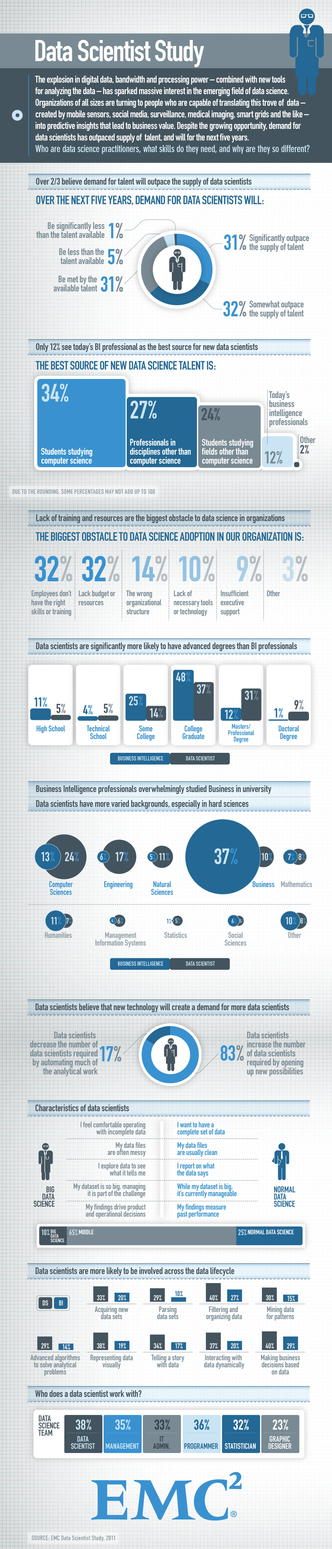
Answer:
I think the “What is a Data Scientist” chart is relatively hard to read and follow for two different reasons: 1) there is too much information on one page -> maybe the author could have found a way to summarize a lot of the points and 2) there could have been an effort to have a better color code in the graphs. All of them are similar shades of blue, which makes it harder to follow and to differentiate the different kinds of graphs. Additionally, I believe there could have been some charts (for example the one containing different bubbles with percentages) that could have been structured differently and easier to read. That could have been easily made as a bar chart or stacked chart, and would have been easier to follow for the reader.
Question #5
Briefly (one paragraph) critique the designer’s choices. Would you have made different choices? Why or why not? Note: Link contains a collection of many data graphics, and I don’t expect (or want) you to write a full report on each individual graphic. But each collection shares some common stylistic elements. You should comment on a few things that you notice about the design of the collection.
Charts that explain food in America
Answer: On the link shared above, I think there are some charts that are really good and easy to follow (chart 2 and 4 for example) and other ones that are very hard to follow given 1) the amount of information being shared 2) the display of the information and 3) the colors being used. Some errors I am able to note in the different graphs is for example in chart 11, instead of using millions, we could have used percentages in the pie chart, that way we can understand what percentage of the pie each one represent. If not, maybe doing a bar graph could have been better to read.Additionally on graph 14, there is no legend being included, which makes it hard for us to understand what each different color means. from the graph, we are not able to decipher which are the countries/regions that eat the most meat.