
Define what a genome is, human perspective.
Like the human genome, or the genome of any other living thing, a bacterium also has a genome, defined as the entirety of its hereditary information, usually encoded as a large single molecule of DNA, called a chromosome.

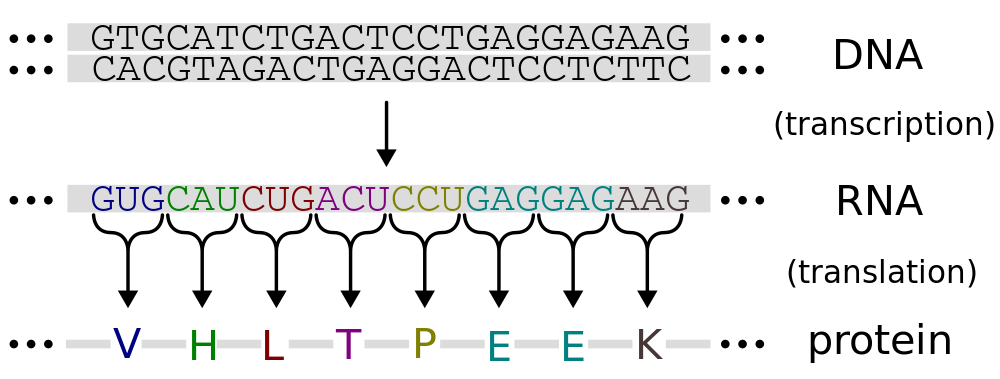
Generally speaking, all other parts of a DNA molecule are identically repeating (especially the sugar-phosphate backbone) except for the precise sequence of its bases. This means the DNA molecule can be effectively represented by a sequence of 4 letters, one for each base, typically A, C, G, T. We will encounter one form or another of this representation of DNA during our analysis in R.
Compared with humans and other Eukaryotes, bacterial genomes are tiny, with sizes ranging from 140 thousand bp to 13 million bp. They most often occur as a single large circular chromosome, often accompanied by one or more much smaller circular DNA molecules called a plasmid.
Unlike humans and other eukaryotes, bacterial and archaeal genomes are mostly (~90%) genes that directly encode proteins. That is, they are informational units that specify a sequence of amino acids in a protein, using a code of 3 letter DNA words. Each 3-letter word in a protein encoding gene sequence specifies one amino acid in the protein sequence.
We are going to use R to look at some features of a bacterial genome, including some protein encoding genes and some genome-wide patterns.
We will be analyzing genome(s) of strains of E.coli, a gram-negative bacterium. I have picked a famous strain of E.coli, called O157:H7, that is often implicated in cases of food-borne illness or swimming in contaminated water.
We will look at some patterns in its genome, and compare with a more wild strain of E.coli if we get the chance.
In this case, information about an E.coli genome has been organized nicely into an R package that contains mostly data. It is available from the biology-specific R repository called Bioconductor, so there are special instructions for installing the package before we can load it and use it.
source("http://bioconductor.org/biocLite.R")
biocLite("BSgenome.Ecoli.NCBI.20080805")
Now that our E.coli genome package has been installed, we can load it with the usual command.
# Load E.coli package
library("BSgenome.Ecoli.NCBI.20080805")
packageVersion("BSgenome.Ecoli.NCBI.20080805")
## [1] '1.3.17'
# look at what data objects are present
ls("package:BSgenome.Ecoli.NCBI.20080805")
## [1] "Ecoli"
# See what one of the sequences is
Ecoli$NC_002695
##   5498450-letter "DNAString" instance
## seq: AGCTTTTCATTCTGACTGCAACGGGCAATATGTC...ACCAAATAAAAAACGCCTTAGTAAGTATTTTTC
# simplify writing this genome later, x now the genome (O157:H7)
x = Ecoli$NC_002695
# E.coli K12
k12 = Ecoli$NC_000913
Alternatively, annotated genome files can be downloaded directly from the NIH ftp site for bacteria. These days it is a huge list that takes a while to load (just the names of the subdirectories, that is).
# E.coli O157:H7 ftp link
ecoli_O157H7_ftp = "ftp://ftp.ncbi.nih.gov/genomes/Bacteria/Escherichia_coli_O157_H7_Sakai_uid57781/NC_002695.gbk"
# E.coli K12 ftp link
ecoli_K12_ftp = "ftp://ftp.ncbi.nih.gov/genomes/Bacteria/Escherichia_coli_K_12_substr__MG1655_uid57779/NC_000913.gbk"
# Save them to temporary files
tempH7 = tempfile()
tempK12 = tempfile()
download.file(ecoli_O157H7_ftp, tempH7)
download.file(ecoli_K12_ftp, tempK12)
# Sequence-only download (if you can't install Bioconductor)
H7_DNAonl_ftp = "ftp://ftp.ncbi.nih.gov/genomes/Bacteria/Escherichia_coli_O157_H7_Sakai_uid57781/NC_002695.fna"
H7ftp = readDNAStringSet(H7_DNAonl_ftp)
H7ftp
##   A DNAStringSet instance of length 1
##       width seq                                        names
## [1] 5498450 AGCTTTTCATTCTGACTGCA...GCCTTAGTAAGTATTTTTC gi|15829254|ref|N...
As discussed in section last week, messenger RNA must have a special sequence of bases for the ribosome to bind, also very close (about 8 bp upstream) to the start codon. In bacteria and archaea, this special sequence is called the Shine-Delgarno sequence. In E.coli, this sequence is exactly AGGAGGU, or AGGAGGT on the chromosome.
Here is some example code for searching the entire genome for just that sequence.
# define a function that counts the number of times a particular word
# appears in a genome
find_count_word = function(x, w, mismatch = 0) {
    # The matches in the forward direction
    for_matches = matchPattern(w, x, max.mismatch = mismatch)
    nfor = length(for_matches@ranges@start)
    # The matches in the reverse direction
    (rpattern = reverseComplement(w))
    rev_matches = matchPattern(rpattern, x, max.mismatch = mismatch)
    nrev = length(rev_matches@ranges@start)
    return(nrev + nfor)
}
find_count_word(x, DNAString("AGGAGGT"))
## [1] 199
# What if we allow one mismatch
find_count_word(x, DNAString("AGGAGGT"), 1)
## [1] 9596
We want to know how the frequency of this sequence compares with other 7-letter words in the E.coli genome.
We can convert this to a testable question:
Does the sequence AGGAGGT occur more often in this E.coli genome than can be explained by chance?
We might guess ahead of time that it does, because Wikipedia told us that it is a special sequence that should occur for nearly every gene, but what do the numbers tell us? How can we test this?
Well, because the word length is relatively short, 7 letters, it is possible to have the computer exhaustively count the frequency of all 7-letter words. In fact, there is a function to do that already
# Count all 7-letter words in genome x
yH7 = oligonucleotideFrequency(x, 7)
So, is our fancy Shine-Delgarno sequence in the top 20 words?
sort(yH7, TRUE)[1:20]
## CGCCAGC GCTGGCG GCCAGCG CGCTGGC CCAGCGC CAGCGCC GCGCTGG CCGCCAG CTGGCGG
##    2442    2418    1893    1872    1853    1835    1827    1789    1776
## GGCGCTG GCCAGCA CTGGCGC TGCTGGC CAGCCAG GCGCCAG CTGGCTG ATCGCCA TGCCAGC
##    1754    1662    1639    1626    1611    1607    1603    1547    1539
## CCAGCAG TTCCAGC
##    1497    1497
Nope. In fact, it doesn't even look close! Did it count our sequence correctly?
yH7["AGGAGGT"]
## AGGAGGT
##      94
# We need to add the count for the reverse complement
yH7["AGGAGGT"] + yH7["ACCTCCT"]
## AGGAGGT
##     199
Well, is it at least a little bit over-represented? Let's build a histogram of the number of times each word appears in the genome (Note: these counts only apply to the forward strand, as written).
hist(yH7)

Well, they don't appear as often as I expected based on the Wikipedia statement. Maybe that was a specific strain of E.coli that has a slightly different Shine-Delgarno sequence.
(1) Pick an instance of the AGGAGGT in the genome
(2) search for a start codon (ATG) 8 to 10 bases downstream on the genome
(3) “read” that hypothetical gene until you hit a stop codon (TAG, TAA, TGA)
(4) Translate the hypothetical gene using the translate function, then copy and paste the hypothetical protein sequence into a public database protein search tool, such as BLASTp
(5) Give me the name of the best match to your discovered protein. Does it do anything that sounds cool?
# I picked the 31st match (you should pick a different one)
matchPattern(DNAString("AGGAGGT"), x, max.mismatch = 0)[31, ]
##   Views on a 5498450-letter DNAString subject
## subject: AGCTTTTCATTCTGACTGCAACGGGCAATATG...CAAATAAAAAACGCCTTAGTAAGTATTTTTC
## views:
##       start     end width
## [1] 1299887 1299893     7 [AGGAGGT]
# This ended at position 1299893, let's look downstream
downstream = x[1299894:(1299893 + 1500)]
# Search for the ATG, the start codon
matchPattern(DNAString("ATG"), downstream, max.mismatch = 0)
##   Views on a 1500-letter DNAString subject
## subject: TTACGACGCTTTTAAAGGTGTGATTCAGGCCA...GTATGGAAATGACCGGGTTAACGTTGTACCG
## views:
##      start  end width
##  [1]    47   49     3 [ATG]
##  [2]    72   74     3 [ATG]
##  [3]   105  107     3 [ATG]
##  [4]   113  115     3 [ATG]
##  [5]   138  140     3 [ATG]
##  [6]   158  160     3 [ATG]
##  [7]   174  176     3 [ATG]
##  [8]   243  245     3 [ATG]
##  [9]   255  257     3 [ATG]
##  ...   ...  ...   ... ...
## [29]  1296 1298     3 [ATG]
## [30]  1326 1328     3 [ATG]
## [31]  1337 1339     3 [ATG]
## [32]  1347 1349     3 [ATG]
## [33]  1362 1364     3 [ATG]
## [34]  1391 1393     3 [ATG]
## [35]  1452 1454     3 [ATG]
## [36]  1472 1474     3 [ATG]
## [37]  1478 1480     3 [ATG]
# The first appears 47 bp downstream! Woops, well, lets use it Did anyone
# find an ATG around 8 bp downstream?  Remove the bases up to that point
downstream = downstream[47:length(downstream)]
aa = translate(downstream)
## Warning: last 2 bases were ignored
aa
##   484-letter "AAString" instance
## seq: MPRRSALLDEVRSKPYWSTDVEMAARAFERYVQD...VRSRLEINKVASVYGTENGKKLKSMEMTGLTLY
as.character(aa)
## [1] "MPRRSALLDEVRSKPYWSTDVEMAARAFERYVQDKARMAGVENDYLVNIRKAPEHNTDNTYAYPTNAELDGGIREAFDHLFRTLKTRETDKGVAFYSRKGVTRTPEGNLISDVNRSAEAKGSPVPQVEAVARGVMSGIKDSDLKVRVVKSQKEAEALAGELFDGYGRVHAFYRPDKREIVLVADNIPDGRTVREKLRHEIIHHAMEHVVTPAEYQTIIKTVLKTRDSDNVTIREAWRKVDASYGKESPEVQAGEFLAHMAEKQPNKFVAAWERVVALVKGVLRRTGLLKPTELNDIRLVRETIRTLGQRVREGYTPREDGAGASFQYSRSGKRDPFKVPEGEGERYRDDLARMMKSLRTTDLTVNIGRTPPVLRHLGAPDLPLVISRDTVRKATNGVKHVVPMDVIERLPELMHDPDAIYRSATERNAVVMLLDAVDKNGDPVVSAVHMKAVRSRLEINKVASVYGTENGKKLKSMEMTGLTLY"
What if that protein sequence was full of stop codons? Well, it would probably not be a real protein-encoding gene. You can still copy the longest stretch without stop codons, and then paste it into a BLASTp search to see what you get. You can also try a different reading frame by removing 1 or 2 bases from the beginning.
For example
downstream = downstream[2:length(downstream)]
aa = translate(downstream)
## Warning: last base was ignored
aa
##   484-letter "AAString" instance
## seq: CRVVQRFSMRCAQNRTGQRMLKWRHVPLSVMFRI...SGRVWKSTR*LLFTVQKMEKN*RVWK*PG*RCT
as.character(aa)
## [1] "CRVVQRFSMRCAQNRTGQRMLKWRHVPLSVMFRIRRVWLAWRMIIWSISVRHLSTTQITPTLIRRMRNWMAVFVRHSITCSAP*KPVRRTRALRFIPVRALPAHLKVISFRMLTVVRKPKAARSRRLKRLPVA**AALRTVT*RSVW*SHRKRLKRWRVNCSMVTAGCTHSIVRINEKLSWWRITSLTGGPFARSCVTRSFTMPWSMLSHQRNIRRLSKPC*KPATVITSPSVKPGVRLMLPMVRNHRKYRRVNFWHIWRRNSRINSWRHGSVLLPWSKGYCVVRGY*SRRN*TISDLFARPSVR*ASVCGKVTRRVRMARAHRFSTPVVVNVIRSKCRKVRASVIVMTLPE**NLCAPQI*R*TSGVRRRYCVTLVHRICRWLFPAILCGRPPMV*NMWCRWMLSRDYRN*CTIRMQFTAQRQKEMRL*CCLMPWIKMVIRWCQRYT*RLSGRVWKSTR*LLFTVQKMEKN*RVWK*PG*RCT"
Go do a public database search of what you find.
The best hit was a known “hypothetical protein ECs1242” in E.coli O157:H7. So we did find a gene, only on the second reading frame that we looked.
FYI, if you're especially interested… There is also a nice review/survey of DNA motif finding algorithms published in BMC Bioinformatics in 2007, it includes many descriptions of alternative scoring functions for evaluating whether a sequence motif is actually over-represented, and how much. This is pretty advanced. Only look a this link if you're especially feeling motivated…
In this particular strain of E.coli, the overall frequency of letters is very close to even.
freq = alphabetFrequency(x)[1:4]
# convert to familiar fractions
freq = freq/sum(freq)
round(freq, 3)
##     A     C     G     T
## 0.248 0.252 0.253 0.247
What about two-letter words?
L = length(x)
# Count the letter frequencies letterFrequencyInSlidingView(x, 2,
# alphabet(x)[1:4])
(di.freq = oligonucleotideFrequency(x, 2))
##     AA     AC     AG     AT     CA     CC     CG     CT     GA     GC
## 403106 303722 283822 370845 384178 321650 399545 280863 319811 444403
##     GG     GT     TA     TC     TG     TT
## 324750 303554 254399 316462 384401 402938
A revealing pattern in bacteria is evident when you look at the frequency of 2-letter words (“dinucleotides”) along the length of the chromosome.
# define window size
w = 50000
s = seq(1, L - w, w)
# e = seq(w, L, 1)
dnw = sapply(s, function(i, x, w) oligonucleotideFrequency(x[i:(i + w - 1)],
    1, TRUE), x, w = 1000)
# re-orient
dnw = t(dnw)
rownames(dnw) = s
head(dnw)
##            A     C     G     T
## 1      0.266 0.260 0.247 0.227
## 50001  0.186 0.247 0.294 0.273
## 100001 0.210 0.246 0.287 0.257
## 150001 0.250 0.241 0.258 0.251
## 200001 0.244 0.224 0.291 0.241
## 250001 0.183 0.304 0.289 0.224
plot(s, dnw[, "C"] + dnw[, "G"], type = "l", xlab = "position", ylab = "C+G")

# First, load ggplot2, show version, and set theme.
library("ggplot2")
packageVersion("ggplot2")
## [1] '0.9.3.1'
theme_set(theme_bw())
data = data.frame(position = s, dnw)
ggplot(data, aes(x = position, y = G + C)) + geom_line()

ggplot(data, aes(x = position, y = A - G)) + geom_line()

There is an interesting method for determining the origin and terminus of replication of a bacterial chromosome using subtle codon bias feature that depends on position relative to these DNA replication regions.
The “ORI” and “TER”, as they are called, can usually be seen graphically with a cumulative walking algorithm, called oriloc, in the seqinr package on CRAN. A small journal article was written about this technique / function.
# Might not work on the latest version of R.
install.packages("sequinr")
# If not, you can download and install from source
install.packages("~/Downloads/seqinr_3.0-6.tar.gz", repos = NULL, type = "source")
Load the new package, and try oriloc.
library("seqinr")

# E.coli-O157:H7
outH7 <- oriloc(gbk = tempH7)
draw.oriloc(outH7)

# E.coli-K12
outK12 <- oriloc(gbk = tempK12)
draw.oriloc(outK12)

There is even a special function for building the transition matrix from the genome, called oligonucleotideTransitions.
oligonucleotideTransitions(x, left = 1, as.prob = TRUE)
##        A      C      G      T
## A 0.2961 0.2231 0.2085 0.2724
## C 0.2771 0.2320 0.2882 0.2026
## G 0.2297 0.3191 0.2332 0.2180
## T 0.1873 0.2330 0.2830 0.2967
oligonucleotideTransitions(x, left = 2, as.prob = TRUE)
##         A      C      G      T
## AA 0.3269 0.2399 0.1859 0.2474
## AC 0.2346 0.2891 0.2804 0.1959
## AG 0.2400 0.3341 0.2159 0.2101
## AT 0.2090 0.2729 0.2476 0.2705
## CA 0.2305 0.2056 0.3263 0.2377
## CC 0.3110 0.1796 0.3214 0.1880
## CG 0.2020 0.3254 0.2597 0.2128
## CT 0.1115 0.1827 0.4415 0.2643
## GA 0.3139 0.2052 0.1631 0.3177
## GC 0.2527 0.2428 0.2932 0.2113
## GG 0.2149 0.3327 0.1817 0.2706
## GT 0.2070 0.2129 0.2625 0.3177
## TA 0.3239 0.2454 0.1233 0.3074
## TC 0.3178 0.2154 0.2551 0.2117
## TG 0.2632 0.2901 0.2620 0.1847
## TT 0.2054 0.2465 0.2206 0.3274
(1) Create a simulated gene using the transition matrix built from the entire E.coli genome.
(2) Translate this gene using the translate function.
(3) Copy and paste the hypothetical protein sequence into a public database protein search tool, such as BLASTp
(4) Repeat, and try to find an interesting-sounding protein. Give me the name of the best match to your discovered protein. Does it do anything that sounds cool?
# Initialize first two bases, using whole genome freq as prior
prior = oligonucleotideFrequency(x, 1, as.prob = TRUE)
first2 = sample(c("A", "C", "G", "T"), 2, TRUE, prob = prior)
first2
## [1] "C" "T"
tranmat = oligonucleotideTransitions(x, left = 2, as.prob = TRUE)
probi = tranmat[paste(first2, collapse = ""), ]
probi
##      A      C      G      T
## 0.1115 0.1827 0.4415 0.2643
next_letter = sample(c("A", "C", "G", "T"), 1, TRUE, prob = probi)
next_letter
## [1] "C"
# Combine the next letter with the previous letters
gene = c(first2, next_letter)
# Now cycle until gene is long enough, e.g. 600 DNA letters
i = 1
while (i < 600) {
    previous2 = gene[(length(gene) - 1):length(gene)]
    probi = tranmat[paste(previous2, collapse = ""), ]
    next_letter = sample(c("A", "C", "G", "T"), 1, TRUE, prob = probi)
    gene = c(gene, next_letter)
    i = i + 1
}
# Now collapse gene as a DNA string
gene_string = DNAString(paste(gene, collapse = ""))
gene_string
##   602-letter "DNAString" instance
## seq: CTCTCGTCACGGCTTTTCAGGCACGATAAAAAGG...CTCTGCGTGTTTCGGGATAACATTCAATTTTGC
aa_string = translate(gene_string)
## Error: 'match' requires vector arguments
aa_string
## Error: object 'aa_string' not found
Some other time, maybe…
Try genoPlotR? You may need to use Mauve for that…
Some other time, maybe…